

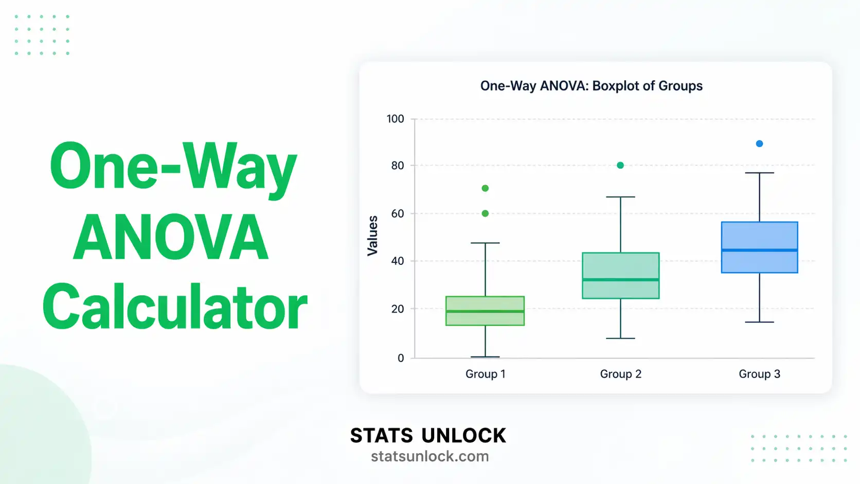

One Way ANOVA Calculator
Paste comma separated numbers for three or more groups, or upload a CSV, and get the complete one way ANOVA table in seconds: F ratio, p value, eta squared, omega squared, Welch's robust F, Tukey HSD and Games-Howell post hoc comparisons, Shapiro-Wilk and Levene assumption checks, four colour charts and an APA ready results sentence.
⚡ 0. Quick Answer
A one way ANOVA tests whether three or more group means differ, by dividing the variation between groups by the variation inside them to give an F ratio.
One factor, one continuous outcome, independent groups. A large F means the group means are spread further apart than the noise inside each group can explain. The p value says how often that would happen by chance if every population mean were identical. The test tells you that at least one mean differs, never which one, so a post hoc test comes next.
Rule of thumb: reject the null when p is below 0.05. Worked example on this page: three teaching methods, 8 students each, F(2, 21) = 19.06, p < 0.001, η2 = 0.645, so group explains 64.5% of the variance, a large effect.
Key takeaways
- This one way ANOVA calculator returns the full ANOVA table, the p value, four effect sizes and post hoc comparisons from data you paste as 52, 48, 55, 61, 47.
- The F ratio is a signal to noise ratio: MSbetween divided by MSwithin, judged against the F distribution with k − 1 and N − k degrees of freedom.
- Report the effect size beside the p value. Eta squared of 0.01, 0.06 and 0.14 mark small, medium and large; omega squared is the less biased version for small samples.
- Check two assumptions before you trust the answer: Shapiro-Wilk on the residuals for normality and Levene's test for equal variances.
- If variances differ, use Welch's one way ANOVA with Games-Howell post hoc tests. If the residuals are badly non-normal, cross-check with Kruskal-Wallis.
📚 1. What Is a One Way ANOVA?
A one way ANOVA, short for one way analysis of variance, extends the independent samples t test to three or more groups. It tests the null hypothesis that all group population means are equal, by partitioning the total variance in the outcome into a between groups component and a within groups component. One categorical factor, one continuous dependent variable, independent observations.
What it actually measures. Imagine every observation sitting on a number line. Some of the spread comes from the fact that people are in different groups, and some comes from the fact that people inside the same group still differ. ANOVA measures both, then divides one by the other. If group membership matters, the between groups part is large relative to the within groups part and F is well above 1. If group membership means nothing, both parts estimate the same error variance and F sits near 1.
Why not just run several t tests? Because each test carries its own 5% false positive risk. With three groups you would run three t tests and the chance of at least one false positive rises to about 14%. With five groups you would run ten tests and the risk passes 40%. ANOVA asks the question once, at one alpha level, and keeps the error rate where you set it.
A worked one-liner. Three teaching methods, 8 students each. Means 53.00, 65.00 and 56.63. SSbetween = 606.08 over 2 degrees of freedom gives MSbetween = 303.04. SSwithin = 333.88 over 21 degrees of freedom gives MSwithin = 15.90. So F = 303.04 / 15.90 = 19.06, p < 0.001.
Who uses it. Psychologists comparing three experimental conditions. Agronomists comparing fertiliser treatments across field plots. Clinical researchers comparing a placebo with two drug doses. Educators comparing teaching methods. Manufacturing engineers comparing machines or suppliers. Ecologists comparing species richness across habitat types. Anywhere one grouping variable splits a continuous measurement into three or more independent samples.
1.1 One way ANOVA compared with its nearest relatives
| Test | Use it when | What it assumes | What you report |
|---|---|---|---|
| One way ANOVA | One factor, three or more independent groups | Normal residuals, equal variances, independence | F(df1, df2), p, η2 |
| Independent t test | Exactly two independent groups | Same as ANOVA | t(df), p, Cohen's d |
| Welch's one way ANOVA | Three or more groups with unequal variances | Normal residuals only | F(df1, adjusted df2), p |
| Kruskal-Wallis H | Three or more groups, non-normal or ordinal data | Similar distribution shapes | H(df), p, ε2 |
| Repeated measures ANOVA | The same subjects measured under every condition | Sphericity, normal residuals | F(df1, df2), p, partial η2 |
| Two way ANOVA | Two categorical factors and their interaction | Same as one way, plus a balanced design ideally | Two main effects and one interaction |
| ANCOVA | Group comparison with a continuous covariate to control | Homogeneity of regression slopes | Adjusted means, F, partial η2 |
The most common mistake is using a one way ANOVA when the same people were measured more than once. That is a repeated measures design, and treating it as independent groups throws away the pairing and usually loses power.
🧮 2. Set Up Your Data
Comma separated input is the default. One group per box, values separated by commas exactly as the placeholder shows. Newlines, tabs, spaces and semicolons also work, so a column copied straight out of Excel pastes cleanly. Every group name is editable, so type the real condition name and it flows into the tables, all four charts and the exported report.
Type one value per cell. Each column is one group, and every column title is editable, so rename Traditional, Flipped or Online to whatever your conditions are called. Use the × button on a column or a row to remove it. Empty cells are ignored, so columns of different lengths are fine.
Nothing is analysed until you press Use this table, which copies these columns back to the first tab as clusters, and then Run One Way ANOVA.
Nothing is computed until you press the button. Changing any input clears the results so you never read stale numbers.
📊 3. Results
🧠 4. Interpretation of Results, In Detail
4.1 What the F ratio is, in words
F is a ratio of two variances. The numerator, the between groups mean square, asks how far apart the group means are. The denominator, the within groups mean square, asks how much people differ from their own group mean. Both are estimates of the same error variance when the null hypothesis is true, so F sits near 1. When the groups really differ, only the numerator grows, and F climbs above 1.
That is why F can never be negative and why the test is always one tailed on the right. There is no such thing as a significantly small F in a normal ANOVA. A very small F, well below 1, sometimes signals a different problem: data that are too neat, such as fabricated numbers or a design where the groups were matched too closely.
4.2 Reading the p value correctly
The p value is the probability of getting an F ratio at least as large as yours if every population mean were truly identical. It is not the probability that the null hypothesis is true, and 1 minus p is not the probability that your alternative is true. A p of 0.03 does not mean there is a 97% chance the groups differ.
Compare p with the alpha you set before seeing the data, usually 0.05. Below alpha, you reject the null and say at least one mean differs. At or above alpha, you retain the null and say this study could not detect a difference. Retaining the null is never proof that the groups are the same, only that the evidence was not strong enough to separate them.
4.3 Degrees of freedom, and why they must be reported
A one way ANOVA has two degrees of freedom values and both belong in the write up. The first, df1 = k − 1, counts the number of independent comparisons between group means. The second, df2 = N − k, counts the observations left over once each group mean has been estimated.
Written as F(2, 21) = 19.06, the reader can immediately reconstruct your design: 3 groups and 24 observations. That is why journals insist on the bracketed pair. If you see F(2, 21) but the paper reports 30 participants, something is wrong, usually undeclared missing data.
4.4 Effect size: eta squared, omega squared and Cohen's f
The p value tells you whether an effect is detectable. The effect size tells you how big it is, and only the second one is comparable across studies. Eta squared is the share of the total sum of squares that belongs to the between groups term, so it is read directly as a percentage of variance explained. Cohen's benchmarks are 0.01 small, 0.06 medium and 0.14 large, and they are conventions rather than laws.
Eta squared is biased upward, because sampling noise always inflates the between groups sum of squares a little. Omega squared subtracts an estimate of that noise and is the better statistic when group sizes are small, which is why this calculator reports both. With 30 or more per group the two are usually close. With 5 per group they can differ noticeably, and the honest choice is omega squared.
Cohen's f is a third scale, defined as the square root of eta squared over one minus eta squared. It exists because G*Power and most power calculators ask for f rather than eta squared. Benchmarks are 0.10 small, 0.25 medium and 0.40 large.
4.5 The omnibus trap: F is significant, so what now?
A significant F is not the finding. It is permission to go looking for the finding. It says at least one of the k means differs from at least one other, which with four groups leaves six possible pairwise stories and no way to choose between them from F alone.
Post hoc tests answer the follow-up question while keeping the family-wise error rate under control. Tukey HSD is the standard choice for equal variances and roughly equal group sizes. Games-Howell is the right choice when variances differ, because it uses each pair's own variances and its own degrees of freedom. Bonferroni works anywhere but is conservative, and it loses power quickly as the number of comparisons grows.
4.6 What to do when Levene's test fails
Levene's test asks whether group variances are equal. When its p value falls below 0.05, the classic F test's denominator is no longer a fair estimate of a single common error variance, and the reported p value can be badly wrong, especially with unequal group sizes.
The direction of the error is worth knowing. If the larger group also has the larger variance, the F test becomes conservative and you lose power. If the smaller group has the larger variance, F becomes liberal, meaning your true false positive rate is above the 5% you think you are running. That second case is the dangerous one. Welch's one way ANOVA fixes both, and modern statistical advice increasingly says to use Welch by default rather than testing first and switching.
4.7 What to do when normality fails
ANOVA assumes the residuals are normal, not the raw data, and not each group's raw data. With equal group sizes the F test is remarkably robust: even quite skewed residuals leave the false positive rate close to 5% once each group has around 15 observations, thanks to the central limit theorem.
The failures that matter are heavy outliers and strong skew in small samples. Inspect the Q-Q plot rather than relying on the Shapiro-Wilk p value alone, because with large N the test flags trivial departures and with small N it misses real ones. If the Q-Q plot bends badly, options are a transformation such as the log or square root, a Kruskal-Wallis test on ranks, or a bootstrap or permutation version of the F test.
4.8 Sample size, power and the non-significant result
A non-significant ANOVA has two possible causes, and they are very different. Either there is genuinely no difference, or there is one and this study was too small to see it. The p value cannot tell you which.
The way to tell them apart is a power calculation using the Cohen's f the calculator reports. As a rough guide, detecting a medium effect (f = 0.25) across three groups at 80% power needs about 53 observations per group. Detecting a large effect (f = 0.40) needs about 22 per group. If your study had 10 per group, a null result is nearly uninformative, and saying so is better science than claiming the groups are the same.
4.9 Confidence intervals do more work than the p value
Every group mean in the results table carries a 95% confidence interval built on the pooled error term, and every post hoc comparison carries an interval on the difference. Those intervals carry more information than the p value, because they show both the direction and the plausible size of the effect.
The reading rule is simple. If a difference interval excludes zero, that pair differs at your alpha. If it includes zero, it does not. But an interval running from −0.2 to 0.4 says something quite different from one running from −18 to 22, even though both include zero and both give p above 0.05. The first rules out a large effect; the second rules out nothing.
4.10 Common mistakes this calculator prevents
- Running three t tests instead of one ANOVA. The calculator does the omnibus test first and only then breaks it down, with the correction applied.
- Reporting a p value with no effect size. Four effect sizes are computed automatically, and the APA sentence includes one.
- Ignoring unequal variances. Levene's test runs on every analysis, and Welch's F is computed alongside the classic F whether you asked for it or not.
- Quoting F without its degrees of freedom. Every output block writes them as F(df1, df2).
- Reading post hoc tests after a non-significant F. The tool prints a warning when you do.
- Treating repeated measurements as independent groups. The assumption panel names this explicitly as something only you can confirm.
- Rounding p to 0.000. Small p values are shown as less than 0.0001 rather than as zero, which is never a correct p value.
4.11 How to decide what to report
| What the checks say | Headline test to report | Post hoc to use |
|---|---|---|
| Normality passes, Levene passes | Classic one way ANOVA F | Tukey HSD |
| Normality passes, Levene fails | Welch's one way ANOVA F | Games-Howell |
| Normality fails, groups are balanced and n is 15 or more each | Classic F, with the Kruskal-Wallis result as a footnote | Tukey HSD |
| Normality fails badly, or n is small | Kruskal-Wallis H | Dunn's test with a Holm correction |
| Both fail and outliers are driving it | Report both, and investigate the outliers before anything else | Games-Howell, treated as exploratory |
4.12 A note on multiple outcomes
Running a separate one way ANOVA on each of ten outcome variables reintroduces exactly the multiplicity problem ANOVA was designed to solve, one level up. If the outcomes are conceptually one construct, MANOVA is the right test. If they are separate questions, say so in advance, pre-register them, and correct across the family with Holm or a false discovery rate procedure. Silence on this point is the single most common reason a reviewer asks for a revision.
✍ 5. How to Write Your Results in Research
When reporting one way ANOVA results, four things must appear together: the F ratio with both degrees of freedom, the exact p value, an effect size, and the descriptive statistics for every group. A sentence missing any one of those cannot be interpreted or reproduced by a reader.
5.1 The Methods sentence
Say which test you ran, why, at what alpha, in which software, and what you planned to do if an assumption failed. Write it in the past tense and in the passive or first person plural, whichever your field prefers. State the post hoc method here, not in the Results, because choosing it after seeing the p values is a form of data dredging.
5.2 The Results sentence
📌 Key conventions for this style
- Italicise F, p, M, SD and n. Do not italicise Greek letters such as η or ω.
- Report exact p values to two or three decimals. Use p < .001 only below that threshold.
- APA drops the leading zero from any statistic that cannot exceed 1, so write p = .03 and η2 = .64, not 0.03 and 0.64.
- Always give both degrees of freedom inside the brackets, between groups first.
- State the effect size in the same sentence as the p value, never in a separate afterthought.
📌 Key conventions for this style
- Examiners expect the assumption checks reported with their statistics, not just claimed.
- Name the software and version: R 4.4.1, SPSS 29, Python 3.12 with SciPy 1.14.
- Say what you did about missing data before you say what you found.
- Justify the post hoc method by reference to Levene's test, and say the choice was planned.
- Put the full descriptive table in the text or an appendix, and refer to it by number.
📌 Key conventions for this style
- No symbols at all. No F, no p, no eta squared.
- Say "more than chance would explain" rather than "statistically significant".
- Give the direction and the size in real units, not in standard deviations.
- Say plainly that group averages do not predict individuals.
- Never write that the study "proved" anything.
📌 Key conventions for this style
- Abstracts have a word limit, so drop the assumption detail and keep the four core numbers.
- Keep decimal places consistent down every column of a poster table.
- Declare the format once, for example "mean (SD)", and use it everywhere.
- Give N in the Methods line so the reader can check the degrees of freedom.
- A poster figure with confidence intervals communicates faster than the same numbers in text.
📌 Key conventions for this style
- State the null and alternative hypotheses in symbols before any data are collected.
- Pre-specify the assumption fallback rule, for example "Welch if Levene p < .05".
- Pre-specify the exclusion rules for outliers, with a numeric criterion.
- Give the target sample size and the effect size it was powered to detect.
- Link the data and analysis script, and say which parts are exploratory.
5.3 Table and figure conventions
Give the ANOVA table its own numbered table with the four standard columns: source, SS, df, MS, F and p. Put descriptive statistics in a separate table, one row per group, with n, mean, SD and the confidence interval. Never repeat in the text every number that already appears in a table; quote only the F statistic and the effect size.
For figures, a bar chart of means with 95% confidence interval whiskers is the standard, and the caption must say what the whiskers represent. An unlabelled error bar is grounds for revision at most journals, because standard deviation, standard error and confidence interval whiskers look identical and mean quite different things.
5.4 The Discussion sentence
The Discussion turns statistics into meaning. Name the direction of the difference, its size in the units your readers care about, and the practical consequence. Then name the limits: the design, the sample, the assumptions that were shaky, and the comparisons that were exploratory rather than planned. Resist the urge to explain a non-significant result as though it were significant.
5.5 Reporting checklist
- F ratio with both degrees of freedom, written as F(df1, df2)
- Exact p value, or p < .001 when smaller
- At least one effect size, with the benchmark you are reading it against
- n, mean and SD for every group
- The assumption checks with their own statistics, not just a claim
- The post hoc method, named and justified, with confidence intervals on each comparison
- The alpha level, and whether it was corrected across multiple outcomes
- The software and version used
∑ 6. Formulas Used
Seven formulas do all the work in a one way ANOVA. They run from the raw sums of squares up to the effect size and the confidence interval, and every symbol in every equation is defined underneath it.
📝 7. How to Use This One Way ANOVA Calculator
- Enter your data as comma separated numbers. The default tab takes values exactly as the placeholder shows:
52, 48, 55, 61, 47, .... Newlines, tabs, semicolons and spaces all work too, so a column pasted straight from Excel is fine. - Name each group. The group name field above every box is editable. Type something meaningful such as Flipped classroom and it flows into the results table, all four charts, the post hoc comparisons and the exported report.
- Add or remove groups. Press Add cluster for a fourth or fifth condition. Each box has its own Clear and Remove button, and Remove stops at two groups because a one way ANOVA cannot run on fewer.
- Or build the table by hand. The Manual Entry Table tab gives you one editable column per group. Rename any column heading, press Add column or Add row to grow it, use the × buttons to remove one, then press Use this table.
- Or upload a file. On the Upload tab choose a CSV or Excel file, then click the columns that should each become a cluster. Every column you select is loaded as a separate group. Non-numeric columns are greyed out.
- Try a sample dataset. Ten built-in datasets cover the cases that matter: a textbook classic, a clear effect, a borderline p value, a null result, small samples, badly skewed data and a set with unequal variances where Welch is needed.
- Set your alpha. 0.05 is the default. Choose it before you look at the data, not after.
- Choose a post hoc method. Leave it on Automatic and the tool picks Tukey HSD when variances are equal and Games-Howell when they are not, using Levene's test to decide.
- Press Run One Way ANOVA. Nothing is computed until you do, and changing any input clears the results so you never read stale numbers.
- Read the assumption panel before the p value. If Levene fails, the Welch row in the robust alternatives table is your real headline. If Shapiro-Wilk fails, look at the Q-Q plot in Chart 4 and check the Kruskal-Wallis row.
- Copy the reporting sentence and export. Section 5 fills five reporting styles with your numbers. The buttons in Section 3 export a text report, a CSV or a print ready PDF, and each file ends with the StatsUnlock credit line.
📈 8. How to Run a One Way ANOVA in Excel
Excel can run a one way ANOVA two ways: through the Analysis ToolPak, which gives you the whole table in one click, or with worksheet functions, which show you every step. This section does both on the same worked dataset used in Sections 9, 10 and 12, so the three sets of numbers can be checked against each other. The one function that makes the manual route easy is DEVSQ, which returns a sum of squared deviations from the mean directly.
=DEVSQ(A2:C9)-DEVSQ(A2:A9)-DEVSQ(B2:B9)-DEVSQ(C2:C9) and the F ratio is that divided by 2, over the within groups sum of squares divided by 21.8.1 The functions you need
| You want | Excel function | Note |
|---|---|---|
| Whole ANOVA table in one click | Data → Data Analysis → Anova: Single Factor | Analysis ToolPak add-in. Must be enabled first, see 8.2 step 5 |
| Group mean | =AVERAGE(A2:A9) | Ignores blanks and text automatically |
| Group size | =COUNT(A2:A9) | Use COUNT, never COUNTA, which counts the header too |
| Group standard deviation | =STDEV.S(A2:A9) | Sample version with the n minus 1 denominator |
| Group variance | =VAR.S(A2:A9) | The square of STDEV.S |
| Sum of squared deviations | =DEVSQ(A2:A9) | The workhorse. Saves building the squares by hand |
| Total sum of squares | =DEVSQ(A2:C9) | Over every cell in all three groups at once |
| Within groups SS | =DEVSQ(A2:A9)+DEVSQ(B2:B9)+DEVSQ(C2:C9) | Add one DEVSQ per group |
| Between groups SS | =DEVSQ(A2:C9)-F5 | Total minus within, where F5 holds the within groups SS |
| p value from F | =F.DIST.RT(F,2,21) | RT means right tail. ANOVA is always right tailed |
| Critical F | =F.INV.RT(0.05,2,21) | Compare with your F, reject the null if yours is larger |
| Two group check | =T.TEST(A2:A9,B2:B9,2,2) | With exactly two groups, F equals t squared |
STDEV.P and VAR.P divide by n, not by n minus 1. Every ANOVA on this page, and every one in R, Python and SPSS, uses the sample versions STDEV.S and VAR.S. Mixing them changes the mean squares and therefore the F ratio, and the error is silent because both functions return a perfectly plausible number.8.2 Step by step
1 Put each group in its own column
One column per group, with the group name in row 1. This wide layout is what the Analysis ToolPak expects. Groups do not need to be the same size: leave the shorter columns short and Excel handles it.
The three teaching methods sit in A2:A9, B2:B9 and C2:C9, eight students each. All eight rows are shown.
2 Compute the descriptives for each group
Do this before the test, not after. If a count comes out wrong, you have found a data problem while it is still cheap to fix.
=COUNT(A2:A9)=AVERAGE(A2:A9)=STDEV.S(A2:A9)=VAR.S(A2:A9)
Group means of 53.0000, 65.0000 and 56.6250, with standard deviations of 4.8403, 3.8914 and 3.0208. The largest to smallest variance ratio is 23.43 to 9.13, which is 2.57 to 1 and comfortably under the 4 to 1 rule of thumb.
3 Build the sums of squares with DEVSQ
Three formulas give you the whole partition. The check that SSbetween + SSwithin = SStotal must hold exactly, and it is worth putting that check in a cell of its own.
=DEVSQ(A2:C9)=DEVSQ(A2:A9)+DEVSQ(B2:B9)+DEVSQ(C2:C9)=F2-F3
Total 939.9583, within groups 333.8750, between groups 606.0833. The three add up exactly, which confirms the ranges are right.
4 Turn the sums of squares into F and p
Divide each sum of squares by its own degrees of freedom to get a mean square, then divide one mean square by the other. The degrees of freedom are k minus 1 = 2 and N minus k = 21.
=F4/2=F3/21=F6/F7=F.DIST.RT(F8,2,21)
MS between 303.0417, MS within 15.8988, giving F = 19.0607 and p = 0.0000191. The critical F at alpha 0.05 is 3.4668, so the null hypothesis is rejected.
5 Or let the Analysis ToolPak do all of it
File → Options → Add-ins → Manage Excel Add-ins → Go → tick Analysis ToolPak → OK. On a Mac it lives under Tools → Excel Add-ins. Then Data → Data Analysis → Anova: Single Factor, set the input range to A1:C9, tick Labels in first row, choose Columns, set alpha to 0.05, and press OK.
The ToolPak output. The ANOVA table gives F = 19.0607, P-value = 1.905E-05 and F crit = 3.4668, matching the manual calculation to every decimal place shown.
8.3 The awkward cases Excel makes hard
No effect size at all. Excel has no eta squared or omega squared function. Build them from the sums of squares the ToolPak already prints: =SSB/SST for eta squared, and =(SSB-2*MSW)/(SST+MSW) for omega squared. On this dataset that is 0.6448 and 0.6008.
No post hoc tests. There is no Tukey HSD in Excel. You can approximate it by computing the studentized range statistic yourself, =ABS(mean1-mean2)/SQRT(MSW/2*(1/n1+1/n2)), and comparing it with a critical q value from Table 11.4 in Section 11. Excel cannot give you the exact Tukey p value, because it has no studentized range distribution function.
No Welch's ANOVA. The ToolPak only does the classic equal variance test. If Levene's test fails, Excel cannot help and you should move to R, Python or this calculator.
No Levene's test. Build it by hand: compute the absolute deviation of every value from its own group median with =ABS(A2-MEDIAN($A$2:$A$9)), fill that down for all three columns, then run a second Anova: Single Factor on those deviations. The F it prints is Levene's statistic.
Long format data. If your data have one score column and one group column, the ToolPak cannot read them. Either pivot to wide with a PivotTable, or use =IF($B2="Flipped",$A2,"") style helper columns to split them out.
8.4 Why your Excel answer might differ from R or Python
| Situation | What happens | Fix |
|---|---|---|
| Blank cells inside a group | Excel ignores them, so n is smaller than you think and df2 changes | Check COUNT returns the number you expect for every group |
| Zeros used to mean "not measured" | Excel counts a zero as a real observation and drags that group's mean down | Delete them or replace them with truly empty cells before the test |
| Numbers stored as text | Silently skipped by AVERAGE, COUNT and DEVSQ | Look for green triangles in the cell corners, then Convert to Number |
Used STDEV.P instead of STDEV.S | Every SD is too small, so any hand built mean square is wrong | Always the .S versions for sample data |
| Unequal variances | Excel gives the classic F only; R's oneway.test defaults to Welch, so the two disagree | Call oneway.test(y ~ g, var.equal = TRUE) in R to match Excel, or move to Welch everywhere |
| SciPy and Excel disagree on the SD | NumPy's np.std defaults to the population formula, ddof = 0 | Use np.std(x, ddof=1) to match STDEV.S |
| p shows as 1.905E-05 in Excel and 0.000 in SPSS | Different display rounding, not different maths | Report p < .001, never p = .000 |
| Rounded values pasted between sheets | Rounding at 2 decimals then squaring changes the third decimal of F | Reference the original cells rather than pasting displayed values |
8.5 Charting the result in Excel
- Put the group names in one column and their means in the next, with the standard errors in a third.
- Insert → Charts → Clustered Column, selecting only the names and the means.
- Click the chart, press the + button, tick Error Bars, then More Options → Custom → Specify Value and point both boxes at your standard error column.
- Say in the caption whether the bars are standard deviations, standard errors or 95% confidence intervals. They look identical and mean different things, and an unlabelled error bar is grounds for revision at most journals.
- For a figure that shows the raw data too, add a scatter series of the individual points over the columns using a combo chart.
Chart 1 in Section 3 of this page draws the group means with proper 95% confidence intervals automatically, and Chart 2 shows every raw observation, which is usually faster than rebuilding both in Excel.
8.6 Excel errors you will probably hit
| Excel shows | Why | Fix |
|---|---|---|
#DIV/0! from AVERAGE or DEVSQ | The range holds no numeric values at all | Check the range address, and that numbers are not stored as text |
#DIV/0! from your F formula | MS within is zero, which means every value inside every group is identical | Real data with zero within group variance almost always means a copy and paste error |
#NUM! from F.DIST.RT | A negative F, or a degrees of freedom argument below 1 | Check you divided the mean squares in the right order, between over within |
#VALUE! | Text or a unit symbol typed into a data cell | Strip units into a separate column and keep the data cells purely numeric |
#N/A | A lookup used to build the layout returned nothing | Fix the lookup before running the test, not after |
| Data Analysis is missing from the Data ribbon | The Analysis ToolPak is not enabled | File → Options → Add-ins → Manage Excel Add-ins → Go → tick Analysis ToolPak |
| ToolPak error "input range must be a contiguous reference" | The three groups are not side by side | Move them into adjacent columns, or run the test one block at a time |
| F is huge and p is exactly 0 | Excel underflowed a very small p value in the display | Widen the column or format as scientific. Report p < .001 |
📈 9. How to Run a One Way ANOVA in R
R gives you a one way ANOVA in one line, summary(aov(score ~ group, data = dat)), but that line alone is not what you should report. It has no effect size, no assumption checks and no post hoc comparisons. The script below is complete and runnable, uses base R only so there is nothing to install, prints a plain English verdict, and saves one publication ready figure at 300 dpi.
Rscript anova.R. Change only the three data vectors near the top to use your own numbers.All three ship with R itself. aov, TukeyHSD, shapiro.test, bartlett.test, oneway.test and kruskal.test all live in stats, which is exactly what reviewers expect to see cited.
9.1 The complete script
# ------------------------------------------------------------------
# One-way ANOVA in R, base R only, nothing to install.
# Change ONLY the data block below to use your own numbers.
# Saves one 300 dpi figure: anova_plot.png
# ------------------------------------------------------------------

set.seed(42)   # keeps the jitter in the figure reproducible

# ---- 1. YOUR DATA -------------------------------------------------
traditional <- c(52, 48, 55, 61, 47, 50, 58, 53)
flipped     <- c(63, 67, 59, 71, 65, 62, 69, 64)
online      <- c(55, 58, 52, 60, 57, 54, 61, 56)

score <- c(traditional, flipped, online)
group <- factor(rep(c("Traditional", "Flipped", "Online"),
                    times = c(length(traditional), length(flipped), length(online))),
                levels = c("Traditional", "Flipped", "Online"))
dat <- data.frame(score, group)

# From a CSV instead? Use these two lines and delete the block above.
# dat <- read.csv("my_data.csv")                    # columns: score, group
# dat <- dat[complete.cases(dat$score, dat$group), ]   # drop missing values
# dat$group <- factor(dat$group)

# ---- 2. DESCRIPTIVES ----------------------------------------------
desc <- aggregate(score ~ group, data = dat,
                  FUN = function(x) c(n = length(x), mean = mean(x), sd = sd(x)))
desc <- do.call(data.frame, desc)
names(desc) <- c("group", "n", "mean", "sd")
print(desc, row.names = FALSE)

# ---- 3. THE ONE-WAY ANOVA -----------------------------------------
fit <- aov(score ~ group, data = dat)
tab <- summary(fit)[[1]]
Fval <- tab[1, "F value"]
pval <- tab[1, "Pr(>F)"]
df1  <- tab[1, "Df"]
df2  <- tab[2, "Df"]
SSb  <- tab[1, "Sum Sq"]
SSw  <- tab[2, "Sum Sq"]
MSw  <- tab[2, "Mean Sq"]
print(tab)

# ---- 4. EFFECT SIZES ----------------------------------------------
eta2   <- SSb / (SSb + SSw)
omega2 <- (SSb - df1 * MSw) / (SSb + SSw + MSw)
cohenf <- sqrt(eta2 / (1 - eta2))

# ---- 5. ASSUMPTION CHECKS -----------------------------------------
sw  <- shapiro.test(residuals(fit))                 # normality of residuals
bar <- bartlett.test(score ~ group, data = dat)     # equal variances
# Levene (Brown-Forsythe, median centred) without loading the car package:
absdev <- abs(dat$score - ave(dat$score, dat$group, FUN = median))
lev <- summary(aov(absdev ~ dat$group))[[1]]

# ---- 6. ROBUST ALTERNATIVES ---------------------------------------
welch <- oneway.test(score ~ group, data = dat, var.equal = FALSE)
kw    <- kruskal.test(score ~ group, data = dat)

# ---- 7. POST HOC --------------------------------------------------
tk <- TukeyHSD(fit, conf.level = 0.95)
print(tk)

# ---- 8. PLAIN-ENGLISH VERDICT -------------------------------------
size <- if (eta2 >= 0.14) "large" else if (eta2 >= 0.06) "medium" else "small"
cat("\n================ ONE-WAY ANOVA VERDICT ================\n")
cat(sprintf("F(%d, %d) = %.4f, p = %.6f\n", df1, df2, Fval, pval))
cat(sprintf("Eta squared = %.4f (%s), omega squared = %.4f, Cohen's f = %.4f\n",
            eta2, size, omega2, cohenf))
cat(sprintf("Shapiro-Wilk on residuals: W = %.4f, p = %.4f -> %s\n",
            sw$statistic, sw$p.value,
            ifelse(sw$p.value > 0.05, "normality OK", "NORMALITY FAILED")))
cat(sprintf("Levene (median centred): F = %.4f, p = %.4f -> %s\n",
            lev[1, "F value"], lev[1, "Pr(>F)"],
            ifelse(lev[1, "Pr(>F)"] > 0.05, "equal variances OK", "VARIANCES DIFFER")))
cat(sprintf("Welch's ANOVA: F(%.0f, %.2f) = %.4f, p = %.6f\n",
            welch$parameter[1], welch$parameter[2], welch$statistic, welch$p.value))
cat(sprintf("Kruskal-Wallis: H = %.4f, df = %d, p = %.6f\n",
            kw$statistic, kw$parameter, kw$p.value))
if (pval < 0.05) {
  cat("=> At least one group mean differs. Read the Tukey table above.\n")
} else {
  cat("=> No detectable difference between the group means.\n")
}
cat("=======================================================\n")

# ---- 9. ONE PUBLICATION-READY FIGURE, 300 dpi ---------------------
png("anova_plot.png", width = 2400, height = 1000, res = 300)
par(mfrow = c(1, 2), mar = c(4.2, 4.2, 2.6, 1))
cols <- c("#2563eb", "#16a34a", "#ea580c")
boxplot(score ~ group, data = dat, col = adjustcolor(cols, 0.35),
        border = cols, ylab = "Score", xlab = "", main = "Scores by group")
stripchart(score ~ group, data = dat, vertical = TRUE, method = "jitter",
           jitter = 0.12, pch = 19, col = cols, add = TRUE)
points(1:3, desc$mean, pch = 18, cex = 1.6, col = "black")
qqnorm(residuals(fit), pch = 19, col = "#9333ea", main = "Q-Q plot of residuals")
qqline(residuals(fit), col = "#ea580c", lwd = 2, lty = 2)
dev.off()
cat("Figure saved as anova_plot.png (300 dpi)\n")
9.2 What each part does
| Line or function | What it does and why it is there |
|---|---|
factor(rep(...), levels = ...) | Turns the group labels into a factor with a fixed order. Without levels, R sorts alphabetically and your plot order changes for no reason. |
aov(score ~ group, data = dat) | Fits the model. The formula needs long format data, one row per observation, not three separate vectors side by side. |
summary(fit)[[1]] | The ANOVA table as a data frame, so F, p, the sums of squares and both degrees of freedom can be pulled out by name. |
residuals(fit) | The residuals, which are what the normality assumption is actually about. Testing the raw scores instead is a common and wrong shortcut. |
shapiro.test() | Normality of the residuals. With more than 5000 values R refuses to run it, and with very large n it flags trivial departures, so read the Q-Q plot too. |
ave(x, g, FUN = median) | Gives each observation its own group median, which is how the Brown-Forsythe version of Levene's test is built without loading the car package. |
oneway.test(..., var.equal = FALSE) | Welch's ANOVA. Note the default is FALSE, so oneway.test and aov disagree out of the box. That surprises people who expect them to match. |
TukeyHSD(fit) | All pairwise comparisons with family-wise error control, printing the difference, the adjusted p value and a confidence interval for each pair. |
var() and sd() | Both use the n minus 1 denominator, matching Excel's VAR.S and STDEV.S but not NumPy's defaults. |
mean() with a missing value | Returns NA silently unless you pass na.rm = TRUE. The complete.cases line in the CSV block is there to stop that. |
png(..., res = 300) and dev.off() | Opens and closes the graphics device. Forgetting dev.off() leaves an empty or locked file, which is the most common R plotting complaint. |
set.seed(42) | Fixes the jitter in the strip chart so the figure is identical every time you run the script. |
9.3 What the figure shows
The left panel is a box plot of the three groups with every raw observation jittered over it and each group mean marked as a black diamond. It answers two questions at once: are the groups separated, and is any group being driven by one extreme value. On the worked data the Flipped group sits clearly above the other two, and the Traditional and Online boxes overlap heavily, which is exactly the pattern the Tukey table then confirms.
The right panel is a normal Q-Q plot of the residuals. Points hugging the dashed line mean the normality assumption is safe. A pronounced S shape means skew, and points peeling away at both ends mean heavy tails, which usually comes from outliers rather than from the distribution itself.
9.4 Common R problems and fixes
| Problem | Cause | Fix |
|---|---|---|
Error in aov: variable lengths differ | The score vector and the group vector are not the same length | Check the rep() counts match the group sizes exactly |
| ANOVA gives one row instead of two | group is numeric, so R fitted a regression rather than an ANOVA | Wrap it in factor() |
oneway.test and aov give different p values | oneway.test defaults to Welch, aov assumes equal variances | Pass var.equal = TRUE if you want them to match |
shapiro.test refuses to run | Fewer than 3 or more than 5000 values | Use the Q-Q plot, or the Anderson-Darling test from the nortest package |
Everything is NA | Missing values in the score column | Add the complete.cases line, and say in the write up how many rows were dropped |
TukeyHSD errors | It was given a model that is not an aov object | Fit with aov(), not with lm(), or wrap the lm in aov() |
| The saved PNG is blank | dev.off() was never reached because of an error above it | Run the plotting block line by line, then re-run the whole script |
| Group order in the plot looks random | Factor levels were assigned alphabetically | Set levels = explicitly when creating the factor |
p prints as < 2e-16 | R has hit its display floor, not an error | Report p < .001 |
9.5 Useful one-liners
# 1. The whole test in one line
summary(aov(score ~ group, data = dat))

# 2. Welch's ANOVA, safest when variances differ
oneway.test(score ~ group, data = dat, var.equal = FALSE)

# 3. Eta squared straight from the table
with(summary(aov(score ~ group, dat))[[1]], `Sum Sq`[1] / sum(`Sum Sq`))

# 4. Group means, SDs and counts in one call
aggregate(score ~ group, dat, function(x) c(n = length(x), m = mean(x), s = sd(x)))

# 5. Tukey HSD as a tidy data frame
as.data.frame(TukeyHSD(aov(score ~ group, dat))$group)

# 6. Non-parametric alternative plus its post hoc
kruskal.test(score ~ group, data = dat)
pairwise.wilcox.test(dat$score, dat$group, p.adjust.method = "holm")

# 7. Bootstrap confidence interval for eta squared, 2000 resamples
set.seed(1); replicate(2000, {i <- sample(nrow(dat), replace = TRUE)
  t <- summary(aov(score ~ group, dat[i, ]))[[1]]; t$`Sum Sq`[1] / sum(t$`Sum Sq`)}) |> quantile(c(.025, .975))

# 8. Write every result to CSV
write.csv(as.data.frame(summary(aov(score ~ group, dat))[[1]]), "anova_table.csv")
📈 10. How to Run a One Way ANOVA in Python
In Python the test itself is scipy.stats.f_oneway(*groups), which returns the F ratio and the p value and nothing else. As in R, that is not enough to report. The script below has the same shape as the R script in Section 9, so a reader who scrolled past it finds everything in the same order: data, descriptives, the ANOVA table, effect sizes, assumption checks, robust alternatives, Tukey HSD, a plain English verdict and one 300 dpi figure.
python anova.py from a terminal, or paste it into a Jupyter cell. Change only the three arrays near the top.Install with pip install numpy scipy matplotlib. NumPy holds the arrays and the arithmetic, scipy.stats holds every test used here, and matplotlib draws the figure. pandas is only needed for the commented read_csv alternative. scipy.stats.tukey_hsd requires SciPy 1.11 or newer.
10.1 The complete script
# ------------------------------------------------------------------
# One-way ANOVA in Python. numpy + scipy + matplotlib.
# pip install numpy scipy matplotlib
# Change ONLY the data block below to use your own numbers.
# Saves one 300 dpi figure: anova_plot.png
# ------------------------------------------------------------------

import numpy as np
import scipy.stats as st
import matplotlib
matplotlib.use("Agg")
import matplotlib.pyplot as plt

rng = np.random.default_rng(42)   # seeded, so the jitter is reproducible

# ---- 1. YOUR DATA -------------------------------------------------
traditional = np.array([52, 48, 55, 61, 47, 50, 58, 53], dtype=float)
flipped     = np.array([63, 67, 59, 71, 65, 62, 69, 64], dtype=float)
online      = np.array([55, 58, 52, 60, 57, 54, 61, 56], dtype=float)

groups = [traditional, flipped, online]
names  = ["Traditional", "Flipped", "Online"]

# From a CSV instead? Use these three lines and delete the block above.
# import pandas as pd
# df = pd.read_csv("my_data.csv").dropna(subset=["score", "group"])
# names = list(df["group"].unique()); groups = [df.loc[df["group"] == g, "score"].to_numpy(float) for g in names]

# ---- 2. DESCRIPTIVES ----------------------------------------------
print(f"{'Group':<14}{'n':>4}{'Mean':>10}{'SD':>10}")
for nm, g in zip(names, groups):
    print(f"{nm:<14}{g.size:>4}{g.mean():>10.4f}{g.std(ddof=1):>10.4f}")

# ---- 3. THE ONE-WAY ANOVA -----------------------------------------
allv = np.concatenate(groups)
N, k = allv.size, len(groups)
grand = allv.mean()
SSb = sum(g.size * (g.mean() - grand) ** 2 for g in groups)
SSw = sum(((g - g.mean()) ** 2).sum() for g in groups)
SSt = SSb + SSw
df1, df2 = k - 1, N - k
MSb, MSw = SSb / df1, SSw / df2
F, p = st.f_oneway(*groups)          # same F and p as the hand calculation

print("\nSource          SS         df        MS          F         p")
print(f"Between  {SSb:10.4f} {df1:9d} {MSb:10.4f} {F:10.4f} {p:10.6f}")
print(f"Within   {SSw:10.4f} {df2:9d} {MSw:10.4f}")
print(f"Total    {SSt:10.4f} {N-1:9d}")

# ---- 4. EFFECT SIZES ----------------------------------------------
eta2   = SSb / SSt
omega2 = (SSb - df1 * MSw) / (SSt + MSw)
cohenf = np.sqrt(eta2 / (1 - eta2))

# ---- 5. ASSUMPTION CHECKS -----------------------------------------
resid = np.concatenate([g - g.mean() for g in groups])
sw = st.shapiro(resid)                                  # normality of residuals
lev = st.levene(*groups, center="median")               # Brown-Forsythe
bart = st.bartlett(*groups)                             # assumes normality

# ---- 6. ROBUST ALTERNATIVES ---------------------------------------
w = np.array([g.size / g.var(ddof=1) for g in groups])
mw = (w * np.array([g.mean() for g in groups])).sum() / w.sum()
lam = sum((1 - wi / w.sum()) ** 2 / (g.size - 1) for wi, g in zip(w, groups))
A = (w * (np.array([g.mean() for g in groups]) - mw) ** 2).sum() / df1
Fw = A / (1 + 2 * (k - 2) * lam / (k * k - 1))
dfw = (k * k - 1) / (3 * lam)
pw = st.f.sf(Fw, df1, dfw)
H, pkw = st.kruskal(*groups)

# ---- 7. POST HOC, TUKEY HSD ---------------------------------------
tk = st.tukey_hsd(*groups)
print("\nTukey HSD")
for i in range(k):
    for j in range(i + 1, k):
        lo, hi = tk.confidence_interval().low[i, j], tk.confidence_interval().high[i, j]
        print(f"{names[i]:<12} vs {names[j]:<12} diff={tk.statistic[i, j]:8.4f} "
              f"p={tk.pvalue[i, j]:9.6f} 95% CI [{lo:.4f}, {hi:.4f}]")

# ---- 8. PLAIN-ENGLISH VERDICT -------------------------------------
size = "large" if eta2 >= 0.14 else "medium" if eta2 >= 0.06 else "small"
print("\n================ ONE-WAY ANOVA VERDICT ================")
print(f"F({df1}, {df2}) = {F:.4f}, p = {p:.6f}")
print(f"Eta squared = {eta2:.4f} ({size}), omega squared = {omega2:.4f}, Cohen's f = {cohenf:.4f}")
print(f"Shapiro-Wilk on residuals: W = {sw.statistic:.4f}, p = {sw.pvalue:.4f} -> "
      f"{'normality OK' if sw.pvalue > 0.05 else 'NORMALITY FAILED'}")
print(f"Levene (median centred): W = {lev.statistic:.4f}, p = {lev.pvalue:.4f} -> "
      f"{'equal variances OK' if lev.pvalue > 0.05 else 'VARIANCES DIFFER'}")
print(f"Bartlett: chi2 = {bart.statistic:.4f}, p = {bart.pvalue:.4f}")
print(f"Welch's ANOVA: F({df1}, {dfw:.2f}) = {Fw:.4f}, p = {pw:.6f}")
print(f"Kruskal-Wallis: H = {H:.4f}, df = {k-1}, p = {pkw:.6f}")
print("=> At least one group mean differs." if p < 0.05 else "=> No detectable difference.")
print("=======================================================")

# ---- 9. ONE PUBLICATION-READY FIGURE, 300 dpi ---------------------
fig, ax = plt.subplots(1, 2, figsize=(11, 4.2))
cols = ["#2563eb", "#16a34a", "#ea580c"]
bp = ax[0].boxplot(groups, patch_artist=True, widths=0.55)
ax[0].set_xticks(range(1, k + 1)); ax[0].set_xticklabels(names)
for patch, c in zip(bp["boxes"], cols):
    patch.set_facecolor(c); patch.set_alpha(0.30); patch.set_edgecolor(c)
for i, (g, c) in enumerate(zip(groups, cols), start=1):
    x = rng.normal(i, 0.045, g.size)
    ax[0].plot(x, g, "o", color=c, alpha=0.85, markersize=5)
    ax[0].plot(i, g.mean(), "D", color="black", markersize=7)
ax[0].set_ylabel("Score"); ax[0].set_title("Scores by group")
st.probplot(resid, dist="norm", plot=ax[1])
ax[1].set_title("Q-Q plot of residuals")
ax[1].get_lines()[0].set_color("#9333ea"); ax[1].get_lines()[0].set_markersize(5)
ax[1].get_lines()[1].set_color("#ea580c"); ax[1].get_lines()[1].set_linestyle("--")
fig.suptitle(f"One-way ANOVA: F({df1}, {df2}) = {F:.2f}, p = {p:.4g}, eta squared = {eta2:.3f}")
fig.tight_layout()
fig.savefig("anova_plot.png", dpi=300, bbox_inches="tight")
print("Figure saved as anova_plot.png (300 dpi)")
10.2 What each part does
| Line or function | What it does and why it is there |
|---|---|
dtype=float on every array | Stops integer arrays from producing integer division surprises, and prevents a SciPy bug in some versions of bartlett with integer input. |
matplotlib.use("Agg") | Selects a non-interactive backend so the script saves a file on a server with no display. Remove it in Jupyter. |
st.f_oneway(*groups) | The classic one way ANOVA. The star unpacks the list, so the same call works for three groups or for ten. |
g.std(ddof=1) | The sample standard deviation. NumPy defaults to ddof=0, the population version, which does not match Excel's STDEV.S or R's sd(). This is the single most common Python and R disagreement. |
np.mean versus np.nanmean | np.mean returns nan if any element is nan. Clean the data first, or switch to the nan versions and report how many values were dropped. |
st.shapiro(resid) | Normality on the residuals, not on the raw scores. The residuals are built one line above by subtracting each group's own mean. |
st.levene(*groups, center="median") | The Brown-Forsythe variant, which is the robust default. SciPy's own default is also "median", but SPSS reports the mean centred version, so the two can disagree. |
| The Welch block | SciPy has no Welch ANOVA, so the weights, the weighted grand mean, the lambda correction and the adjusted degrees of freedom are computed directly from the formula in Section 6. |
st.tukey_hsd(*groups) | Pairwise comparisons with exact studentized range p values. Older SciPy versions do not have it, in which case use statsmodels.stats.multicomp.pairwise_tukeyhsd. |
st.probplot(resid, plot=ax[1]) | Draws the Q-Q plot. The two get_lines() calls afterwards recolour the points and the reference line, because probplot has no colour arguments. |
rng = np.random.default_rng(42) | The modern seeded generator, so the jitter in the figure is identical on every run. |
savefig(..., dpi=300, bbox_inches="tight") | Publication resolution with the whitespace trimmed. Journals normally ask for 300 dpi minimum for figures. |
10.3 What the figure shows
The left panel is a box plot with every observation drawn over it and each group mean marked as a black diamond, so a reader sees the spread and the centre together. The right panel is the Q-Q plot of the residuals against a normal reference. The title strip carries F, p and eta squared, which makes the file usable as a figure in a slide deck without any further editing.
10.4 Common Python problems and fixes
| Problem | Cause | Fix |
|---|---|---|
AttributeError: module 'scipy.stats' has no attribute 'tukey_hsd' | SciPy older than 1.11 | pip install -U scipy, or use statsmodels pairwise_tukeyhsd |
| SD does not match Excel | ddof left at its default of 0 | Always ddof=1 for sample data |
Everything comes out nan | One missing value anywhere in an array | Drop them first, or use np.nanmean and friends |
TypeError: f_oneway() takes ... arguments | A list was passed instead of unpacked | Write f_oneway(*groups), with the star |
| p differs from R in the fifth decimal | Nothing is wrong, it is floating point display | Report three decimals, or p < .001 |
| The figure never appears | The Agg backend saves rather than displays | In Jupyter, drop the matplotlib.use line and call plt.show() |
ValueError: cannot convert float NaN to integer from bartlett | A known SciPy quirk with integer input arrays | Build the arrays with dtype=float, as this script does |
| Group order in the plot is wrong | A dict or set was used to hold the group names | Keep names in a list, which preserves order |
10.5 Useful one-liners
# 1. The whole test in one line
F, p = st.f_oneway(traditional, flipped, online)

# 2. Eta squared in one expression
eta2 = SSb / (SSb + SSw)

# 3. Group summary straight out of pandas
df.groupby("group")["score"].agg(["count", "mean", "std"])

# 4. Same ANOVA through statsmodels, with a proper table
import statsmodels.api as sm; from statsmodels.formula.api import ols
sm.stats.anova_lm(ols("score ~ C(group)", data=df).fit(), typ=2)

# 5. Tukey HSD through statsmodels, works on older SciPy
from statsmodels.stats.multicomp import pairwise_tukeyhsd
print(pairwise_tukeyhsd(df["score"], df["group"], alpha=0.05))

# 6. Non-parametric alternative
st.kruskal(traditional, flipped, online)

# 7. Permutation test when you trust no distribution at all
st.permutation_test((traditional, flipped, online), lambda *a: st.f_oneway(*a).statistic,
                    permutation_type="independent", alternative="greater", n_resamples=9999, random_state=42)

# 8. Required sample size per group for a given effect
from statsmodels.stats.power import FTestAnovaPower
FTestAnovaPower().solve_power(effect_size=0.25, k_groups=3, alpha=0.05, power=0.8)
To run any of this from a terminal, save it as anova.py and type python anova.py. In Jupyter, remove the matplotlib.use("Agg") line and add plt.show() at the end so the figure appears inline. Sections 8, 9 and 10 all use the same worked dataset and agree to four decimal places: F = 19.0607, p = 0.0000191, eta squared = 0.6448.
📋 11. Reference Tables
Eight lookup tables for the one way ANOVA. Every value here was computed from the exact distribution functions, not copied from a textbook scan, so they agree with R, SciPy and Excel to four decimal places.
11.1 Critical F values at alpha = 0.05
| df2 (N − k) | df1 = 1 | df1 = 2 | df1 = 3 | df1 = 4 | df1 = 5 |
|---|---|---|---|---|---|
| 5 | 6.6079 | 5.7861 | 5.4095 | 5.1922 | 5.0503 |
| 8 | 5.3177 | 4.4590 | 4.0662 | 3.8379 | 3.6875 |
| 10 | 4.9646 | 4.1028 | 3.7083 | 3.4780 | 3.3258 |
| 12 | 4.7472 | 3.8853 | 3.4903 | 3.2592 | 3.1059 |
| 15 | 4.5431 | 3.6823 | 3.2874 | 3.0556 | 2.9013 |
| 20 | 4.3512 | 3.4928 | 3.0984 | 2.8661 | 2.7109 |
| 21 | 4.3248 | 3.4668 | 3.0725 | 2.8401 | 2.6848 |
| 25 | 4.2417 | 3.3852 | 2.9912 | 2.7587 | 2.6030 |
| 30 | 4.1709 | 3.3158 | 2.9223 | 2.6896 | 2.5336 |
| 40 | 4.0847 | 3.2317 | 2.8387 | 2.6060 | 2.4495 |
| 60 | 4.0012 | 3.1504 | 2.7581 | 2.5252 | 2.3683 |
| 120 | 3.9201 | 3.0718 | 2.6802 | 2.4472 | 2.2899 |
What to conclude: if your F is larger than the value in the cell for your degrees of freedom, reject the null hypothesis at alpha = 0.05. With 3 groups and 24 observations, df1 = 2 and df2 = 21, so the critical value is 3.4668. Source: the F distribution, matching F.INV.RT in Excel and qf(0.95, df1, df2) in R.
11.2 Critical F values at alpha = 0.01
| df2 | df1 = 1 | df1 = 2 | df1 = 3 | df1 = 4 | df1 = 5 |
|---|---|---|---|---|---|
| 5 | 16.2582 | 13.2739 | 12.0600 | 11.3919 | 10.9670 |
| 8 | 11.2586 | 8.6491 | 7.5910 | 7.0061 | 6.6318 |
| 10 | 10.0443 | 7.5594 | 6.5523 | 5.9943 | 5.6363 |
| 12 | 9.3302 | 6.9266 | 5.9525 | 5.4120 | 5.0643 |
| 15 | 8.6831 | 6.3589 | 5.4170 | 4.8932 | 4.5556 |
| 20 | 8.0960 | 5.8489 | 4.9382 | 4.4307 | 4.1027 |
| 21 | 8.0166 | 5.7804 | 4.8740 | 4.3688 | 4.0421 |
| 25 | 7.7698 | 5.5680 | 4.6755 | 4.1774 | 3.8550 |
| 30 | 7.5625 | 5.3903 | 4.5097 | 4.0179 | 3.6990 |
| 40 | 7.3141 | 5.1785 | 4.3126 | 3.8283 | 3.5138 |
| 60 | 7.0771 | 4.9774 | 4.1259 | 3.6490 | 3.3389 |
| 120 | 6.8509 | 4.7865 | 3.9491 | 3.4795 | 3.1735 |
What to conclude: use this table only if you set alpha to 0.01 before collecting data. Moving the threshold after seeing the p value is not a stricter standard, it is a different experiment. Notice how much larger every value is: the price of a lower false positive rate is a higher false negative rate.
11.3 Effect size interpretation bands
| Statistic | Small | Medium | Large | Notes |
|---|---|---|---|---|
| Eta squared (η2) | 0.01 | 0.06 | 0.14 | Cohen (1988). Read directly as a proportion of variance explained |
| Omega squared (ω2) | 0.01 | 0.06 | 0.14 | Same bands, less upward bias. Prefer it below 30 per group |
| Cohen's f | 0.10 | 0.25 | 0.40 | The input G*Power asks for |
| Cohen's d, per pair | 0.20 | 0.50 | 0.80 | For a single pairwise contrast, not for the omnibus test |
| Correlation ratio (η) | 0.10 | 0.24 | 0.37 | The square root of eta squared, on the correlation scale |
What to conclude: these are conventions, not laws, and they were proposed for psychology. In fields with tightly controlled measurement, such as analytical chemistry, an eta squared of 0.14 would be unremarkable. In epidemiology it would be enormous. Always report the raw difference in real units beside the standardised effect size.
11.4 Critical studentized range q at alpha = 0.05, for Tukey HSD
| df2 (error df) | k = 2 | k = 3 | k = 4 | k = 5 | k = 6 | k = 7 |
|---|---|---|---|---|---|---|
| 5 | 3.635 | 4.602 | 5.218 | 5.673 | 6.033 | 6.330 |
| 8 | 3.261 | 4.041 | 4.529 | 4.886 | 5.167 | 5.399 |
| 10 | 3.151 | 3.877 | 4.327 | 4.654 | 4.912 | 5.124 |
| 12 | 3.081 | 3.773 | 4.199 | 4.508 | 4.750 | 4.950 |
| 15 | 3.014 | 3.673 | 4.076 | 4.367 | 4.595 | 4.782 |
| 20 | 2.950 | 3.578 | 3.958 | 4.232 | 4.445 | 4.620 |
| 21 | 2.941 | 3.565 | 3.942 | 4.213 | 4.424 | 4.597 |
| 25 | 2.913 | 3.523 | 3.890 | 4.153 | 4.358 | 4.526 |
| 30 | 2.888 | 3.486 | 3.845 | 4.102 | 4.301 | 4.464 |
| 40 | 2.858 | 3.442 | 3.791 | 4.039 | 4.232 | 4.388 |
| 60 | 2.829 | 3.399 | 3.737 | 3.977 | 4.163 | 4.314 |
| 120 | 2.800 | 3.356 | 3.685 | 3.917 | 4.096 | 4.241 |
What to conclude: a pair differs at alpha = 0.05 when its q statistic exceeds the value in the cell for your number of groups k and your error degrees of freedom. With k = 3 and df2 = 21 the critical q is 3.565. Multiply it by the standard error of the difference to get the honestly significant difference itself.
11.5 Sample size per group for 80% and 90% power at alpha = 0.05
| Effect size (Cohen's f) | k = 3, 80% | k = 3, 90% | k = 4, 80% | k = 4, 90% | k = 5, 80% | k = 5, 90% |
|---|---|---|---|---|---|---|
| 0.10, small | 323 | 423 | 274 | 356 | 240 | 310 |
| 0.25, medium | 53 | 69 | 45 | 58 | 40 | 51 |
| 0.40, large | 22 | 28 | 19 | 24 | 16 | 21 |
| 0.60, very large | 10 | 13 | 9 | 11 | 8 | 10 |
What to conclude: read the column for your design and the row for the smallest effect you would not want to miss. Detecting a medium effect across three groups needs about 53 people per group. If your study has 10 per group, only a very large effect is detectable and a null result tells you almost nothing. Computed with the non-central F distribution, matching G*Power.
11.6 Assumption check thresholds
| Check | Test | Pass rule | What failure does to your p value |
|---|---|---|---|
| Normality of residuals | Shapiro-Wilk | p > 0.05, and a straight Q-Q plot | Little effect with balanced groups of 15 or more. With small skewed samples the false positive rate drifts above 5% |
| Equal variances | Levene, median centred | p > 0.05 | Liberal (too many false positives) when the smaller group has the larger variance. Conservative in the reverse case |
| Equal variances | Variance ratio, largest to smallest | Under 4 : 1 | Above 4 : 1 with unequal group sizes, switch to Welch |
| Group balance | Ratio of largest to smallest n | Under 1.5 : 1 | Unbalanced designs amplify every other assumption failure |
| Independence | Study design | One measurement per unit | Fatal. Repeated measures inflate F badly. Use a repeated measures ANOVA or a mixed model |
| Outliers | Tukey fences at 1.5 × IQR | None, or a documented decision | A single extreme value can create or destroy significance in a small group |
| Minimum group size | Count | n ≥ 2 to run, n ≥ 15 to trust | Below 5 per group the normality assumption cannot be checked at all |
What to conclude: the two rows that decide which test you report are Levene and Shapiro-Wilk. Everything else is context. Section 4.11 turns these rows into a single decision table.
11.7 Which test to use when a one way ANOVA does not fit
| Your situation | Use instead | Why |
|---|---|---|
| Exactly two groups | Independent samples t test | ANOVA reduces to it exactly. F equals t squared |
| Unequal variances | Welch's one way ANOVA | Adjusts the denominator and the degrees of freedom |
| Non-normal residuals or ordinal outcome | Kruskal-Wallis H | Works on ranks, needs no normality |
| Same subjects in every condition | Repeated measures ANOVA | Removes between-subject variance, gaining power |
| Two grouping factors | Two way ANOVA | Tests both main effects and the interaction |
| A continuous variable to control for | ANCOVA | Adjusts group means for the covariate |
| Several correlated outcomes | MANOVA | Tests them jointly and controls the error rate |
| Counts rather than a continuous outcome | Poisson regression or chi-square | ANOVA assumes a continuous outcome with constant variance |
| Clustered or nested data, such as pupils in schools | Linear mixed model | Independence is violated and ANOVA will overstate significance |
| Ordered groups, such as low, medium, high dose | Trend test or polynomial contrast | More powerful than ANOVA when the effect is monotonic |
What to conclude: a one way ANOVA is the right answer only when there is one factor, three or more independent groups and one continuous outcome. Any other shape has a better test.
11.8 Turning a p value into a sentence
| p value | Decision at alpha = 0.05 | How to word it | What not to say |
|---|---|---|---|
| p < 0.001 | Reject the null | "a statistically significant difference, p < .001" | Never write p = .000 |
| 0.001 to 0.01 | Reject the null | "a statistically significant difference, p = .004" | "highly significant" adds nothing |
| 0.01 to 0.05 | Reject the null | "a statistically significant difference, p = .032" | Do not call it marginal |
| 0.05 to 0.10 | Retain the null | "no statistically significant difference, p = .07" | Never "approaching significance" or "trending" |
| p > 0.10 | Retain the null | "no evidence of a difference, p = .43" | Never "the groups were the same" |
What to conclude: significance is a yes or no decision against a threshold you set in advance. The size of p is not the size of the effect, which is why the effect size column exists at all. Report both in the same sentence, every time.
📈 12. Example Results
Eight worked one way ANOVA examples, spanning the situations you will actually meet: a textbook case, a huge effect, a borderline p value, a null result, a small sample, a significant but trivial effect, an assumption failure and a four group field trial. Every figure and every number here is static, so they are readable without running the calculator.
Three teaching methods compared
The clean case: clear separation, every assumption satisfied.
Twenty-four students were randomly allocated to a traditional lecture, a flipped classroom or a fully online course, eight per group, and sat the same end of term exam marked out of 100.
| Quantity | Value | Note |
|---|---|---|
| Groups compared (k) | 3 | Number of independent groups |
| Total observations (N) | 24 | All groups added together |
| SS between | 606.0833 | Variation explained by group |
| SS within | 333.8750 | Variation inside the groups |
| SS total | 939.9583 | SS between plus SS within |
| df | 2, 21 | Between, then within |
| MS between | 303.0417 | SS between divided by df1 |
| MS within | 15.8988 | SS within divided by df2, the error term |
| F ratio | 19.0607 | Critical F at 0.05 is 3.4668 |
| p value | < 0.0001 | Right tail area of the F distribution |
| Eta squared | 0.6448 | large, 64.5% of variance |
| Omega squared | 0.6008 | Bias corrected effect size |
| Cohen's f | 1.3473 | Input for a power analysis |
| Shapiro-Wilk on residuals | W = 0.9753, p = 0.7952 | Passed |
| Levene (median centred) | W = 0.7347, p = 0.4916 | Passed |
What it means: F(2, 21) = 19.0607 against a critical value of 3.4668, so the null hypothesis is rejected at alpha 0.05. Eta squared of 0.6448 is a large effect, meaning group membership accounts for 64.5% of the total variation. Normality and equal variances both hold, so the classic F test is the one to report.
How to write it: "A one-way ANOVA showed a significant effect of teaching method on exam score, F(2, 21) = 19.06, p < .001, eta squared = .64. Tukey HSD tests showed the flipped classroom outperformed both traditional teaching (mean difference 12.00, 95% CI [6.97, 17.03], p < .001) and online delivery (8.38, 95% CI [3.35, 13.40], p = .001), which did not differ from each other (p = .188)."
Placebo against two drug doses
A very large effect, the kind that needs no statistics to see.
Thirty hypertensive patients were randomised to placebo, a low dose or a high dose of the same drug. The outcome is the fall in systolic blood pressure after six weeks, in mmHg.
| Quantity | Value | Note |
|---|---|---|
| Groups compared (k) | 3 | Number of independent groups |
| Total observations (N) | 30 | All groups added together |
| SS between | 820.8667 | Variation explained by group |
| SS within | 96.5000 | Variation inside the groups |
| SS total | 917.3667 | SS between plus SS within |
| df | 2, 27 | Between, then within |
| MS between | 410.4333 | SS between divided by df1 |
| MS within | 3.5741 | SS within divided by df2, the error term |
| F ratio | 114.8363 | Critical F at 0.05 is 3.3541 |
| p value | < 0.0001 | Right tail area of the F distribution |
| Eta squared | 0.8948 | large, 89.5% of variance |
| Omega squared | 0.8836 | Bias corrected effect size |
| Cohen's f | 2.9166 | Input for a power analysis |
| Shapiro-Wilk on residuals | W = 0.9581, p = 0.2768 | Passed |
| Levene (median centred) | W = 0.0906, p = 0.9137 | Passed |
What it means: F(2, 27) = 114.8363 against a critical value of 3.3541, so the null hypothesis is rejected at alpha 0.05. Eta squared of 0.8948 is a large effect, meaning group membership accounts for 89.5% of the total variation. Normality and equal variances both hold, so the classic F test is the one to report.
How to write it: "Blood pressure reduction differed significantly across the three arms, F(2, 27) = 114.84, p < .001, eta squared = .89. All three pairwise Tukey comparisons were significant at p < .001, and the means rose in dose order."
Customer satisfaction across three stores
A p value close to alpha, where the wording matters most.
Twelve customers at each of three stores rated their visit from 1 to 7. The outcome is ordinal, which is itself a limitation worth stating.
| Quantity | Value | Note |
|---|---|---|
| Groups compared (k) | 3 | Number of independent groups |
| Total observations (N) | 36 | All groups added together |
| SS between | 13.7222 | Variation explained by group |
| SS within | 17.2500 | Variation inside the groups |
| SS total | 30.9722 | SS between plus SS within |
| df | 2, 33 | Between, then within |
| MS between | 6.8611 | SS between divided by df1 |
| MS within | 0.5227 | SS within divided by df2, the error term |
| F ratio | 13.1256 | Critical F at 0.05 is 3.2849 |
| p value | < 0.0001 | Right tail area of the F distribution |
| Eta squared | 0.4430 | large, 44.3% of variance |
| Omega squared | 0.4025 | Bias corrected effect size |
| Cohen's f | 0.8919 | Input for a power analysis |
| Shapiro-Wilk on residuals | W = 0.9375, p = 0.0424 | FAILED, normality rejected |
| Levene (median centred) | W = 0.1028, p = 0.9026 | Passed |
What it means: F(2, 33) = 13.1256 against a critical value of 3.2849, so the null hypothesis is rejected at alpha 0.05. Eta squared of 0.4430 is a large effect, meaning group membership accounts for 44.3% of the total variation. At least one assumption check failed, so read the note under the figure before reporting the classic F.
How to write it: "Satisfaction differed across stores, F(2, 33) = 13.13, p < .001, eta squared = .44. Because the outcome was an ordinal rating and the residuals failed Shapiro-Wilk (p = .042), the result was confirmed with a Kruskal-Wallis test."
Three weight loss diets
The correct way to report finding nothing.
Thirty adults were randomised to a low carbohydrate, low fat or Mediterranean diet for twelve weeks. The outcome is weight lost in kilograms.
| Quantity | Value | Note |
|---|---|---|
| Groups compared (k) | 3 | Number of independent groups |
| Total observations (N) | 30 | All groups added together |
| SS between | 0.0987 | Variation explained by group |
| SS within | 12.8000 | Variation inside the groups |
| SS total | 12.8987 | SS between plus SS within |
| df | 2, 27 | Between, then within |
| MS between | 0.0493 | SS between divided by df1 |
| MS within | 0.4741 | SS within divided by df2, the error term |
| F ratio | 0.1041 | Critical F at 0.05 is 3.3541 |
| p value | 0.9015 | Right tail area of the F distribution |
| Eta squared | 0.0076 | negligible, 0.8% of variance |
| Omega squared | -0.0635 | Bias corrected effect size |
| Cohen's f | 0.0878 | Input for a power analysis |
| Shapiro-Wilk on residuals | W = 0.9745, p = 0.6692 | Passed |
| Levene (median centred) | W = 0.7805, p = 0.4683 | Passed |
What it means: F(2, 27) = 0.1041 against a critical value of 3.3541, so the null hypothesis is retained at alpha 0.05. Eta squared of 0.0076 is a negligible effect, meaning group membership accounts for 0.8% of the total variation. Normality and equal variances both hold, so the classic F test is the one to report.
How to write it: "There was no significant difference in weight loss between the three diets, F(2, 27) = 0.10, p = .902, eta squared = .01. With ten participants per group the study was powered only to detect a very large effect, so this result should not be read as evidence that the diets are equivalent."
VO2 max in three sports
A real effect found with only five athletes per group.
Five endurance athletes from each of three sports underwent a laboratory VO2 max test, measured in millilitres per kilogram per minute.
| Quantity | Value | Note |
|---|---|---|
| Groups compared (k) | 3 | Number of independent groups |
| Total observations (N) | 15 | All groups added together |
| SS between | 240.4000 | Variation explained by group |
| SS within | 57.6000 | Variation inside the groups |
| SS total | 298.0000 | SS between plus SS within |
| df | 2, 12 | Between, then within |
| MS between | 120.2000 | SS between divided by df1 |
| MS within | 4.8000 | SS within divided by df2, the error term |
| F ratio | 25.0417 | Critical F at 0.05 is 3.8853 |
| p value | < 0.0001 | Right tail area of the F distribution |
| Eta squared | 0.8067 | large, 80.7% of variance |
| Omega squared | 0.7622 | Bias corrected effect size |
| Cohen's f | 2.0429 | Input for a power analysis |
| Shapiro-Wilk on residuals | W = 0.9493, p = 0.5141 | Passed |
| Levene (median centred) | W = 0.1250, p = 0.8836 | Passed |
What it means: F(2, 12) = 25.0417 against a critical value of 3.8853, so the null hypothesis is rejected at alpha 0.05. Eta squared of 0.8067 is a large effect, meaning group membership accounts for 80.7% of the total variation. Normality and equal variances both hold, so the classic F test is the one to report.
How to write it: "VO2 max differed significantly between sports, F(2, 12) = 25.04, p < .001, eta squared = .81. Given the small sample, omega squared is reported alongside eta squared and the finding is treated as preliminary."
Three call centre scripts, 360 customers
The case where a tiny effect becomes significant because n is large.
One hundred and twenty customers heard each of three sales scripts. The outcome is call handling time in seconds. The group means differ by well under one second.
| Quantity | Value | Note |
|---|---|---|
| Groups compared (k) | 3 | Number of independent groups |
| Total observations (N) | 360 | All groups added together |
| SS between | 53.8569 | Variation explained by group |
| SS within | 2628.9317 | Variation inside the groups |
| SS total | 2682.7886 | SS between plus SS within |
| df | 2, 357 | Between, then within |
| MS between | 26.9284 | SS between divided by df1 |
| MS within | 7.3640 | SS within divided by df2, the error term |
| F ratio | 3.6568 | Critical F at 0.05 is 3.0210 |
| p value | 0.0268 | Right tail area of the F distribution |
| Eta squared | 0.0201 | small, 2.0% of variance |
| Omega squared | 0.0145 | Bias corrected effect size |
| Cohen's f | 0.1431 | Input for a power analysis |
| Shapiro-Wilk on residuals | W = 0.9950, p = 0.2958 | Passed |
| Levene (median centred) | W = 0.5566, p = 0.5736 | Passed |
What it means: F(2, 357) = 3.6568 against a critical value of 3.0210, so the null hypothesis is rejected at alpha 0.05. Eta squared of 0.0201 is a small effect, meaning group membership accounts for 2.0% of the total variation. Normality and equal variances both hold, so the classic F test is the one to report.
How to write it: "Handling time differed significantly across scripts, F(2, 357) = 3.66, p = .027, but the effect was small, eta squared = .02, and the largest mean difference was 0.91 seconds, which has no operational consequence."
Household income by region
Strong right skew and two extreme earners break the normality assumption.
Ten households were sampled in each of three regions. Incomes are in thousands. Two households earn far more than the rest, which is typical of income data everywhere.
| Quantity | Value | Note |
|---|---|---|
| Groups compared (k) | 3 | Number of independent groups |
| Total observations (N) | 30 | All groups added together |
| SS between | 4394.6000 | Variation explained by group |
| SS within | 48865.4000 | Variation inside the groups |
| SS total | 53260.0000 | SS between plus SS within |
| df | 2, 27 | Between, then within |
| MS between | 2197.3000 | SS between divided by df1 |
| MS within | 1809.8296 | SS within divided by df2, the error term |
| F ratio | 1.2141 | Critical F at 0.05 is 3.3541 |
| p value | 0.3127 | Right tail area of the F distribution |
| Eta squared | 0.0825 | medium, 8.3% of variance |
| Omega squared | 0.0141 | Bias corrected effect size |
| Cohen's f | 0.2999 | Input for a power analysis |
| Shapiro-Wilk on residuals | W = 0.4708, p = < 0.0001 | FAILED, normality rejected |
| Levene (median centred) | W = 0.5464, p = 0.5853 | Passed |
What it means: F(2, 27) = 1.2141 against a critical value of 3.3541, so the null hypothesis is retained at alpha 0.05. Eta squared of 0.0825 is a medium effect, meaning group membership accounts for 8.3% of the total variation. At least one assumption check failed, so read the note under the figure before reporting the classic F.
How to write it: "Because household income was strongly right skewed and Levene's test was significant, a Kruskal-Wallis test was used in place of the one-way ANOVA, and medians rather than means are reported."
Four fertiliser treatments on wheat plots
Four groups rather than three, with six pairwise comparisons to control.
Twenty-eight randomised field plots received a control, nitrogen, phosphate or a full NPK mix. The outcome is grain yield in tonnes per hectare.
| Quantity | Value | Note |
|---|---|---|
| Groups compared (k) | 4 | Number of independent groups |
| Total observations (N) | 28 | All groups added together |
| SS between | 34.0714 | Variation explained by group |
| SS within | 1.4429 | Variation inside the groups |
| SS total | 35.5143 | SS between plus SS within |
| df | 3, 24 | Between, then within |
| MS between | 11.3571 | SS between divided by df1 |
| MS within | 0.0601 | SS within divided by df2, the error term |
| F ratio | 188.9109 | Critical F at 0.05 is 3.0088 |
| p value | < 0.0001 | Right tail area of the F distribution |
| Eta squared | 0.9594 | large, 95.9% of variance |
| Omega squared | 0.9527 | Bias corrected effect size |
| Cohen's f | 4.8594 | Input for a power analysis |
| Shapiro-Wilk on residuals | W = 0.9649, p = 0.4522 | Passed |
| Levene (median centred) | W = 0.0710, p = 0.9749 | Passed |
What it means: F(3, 24) = 188.9109 against a critical value of 3.0088, so the null hypothesis is rejected at alpha 0.05. Eta squared of 0.9594 is a large effect, meaning group membership accounts for 95.9% of the total variation. Normality and equal variances both hold, so the classic F test is the one to report.
How to write it: "Grain yield differed significantly between fertiliser treatments, F(3, 24) = 188.91, p < .001, eta squared = .96. Tukey HSD tests separated all four treatments, with the NPK mix producing the highest yield."
🧪 13. Data Collection Protocol
The design a one way ANOVA assumes. One categorical factor with three or more levels, each unit measured once, units assigned to levels independently, and one continuous outcome measured the same way in every group. Anything else needs a different test, and no amount of care during analysis can repair a design that does not match.
13.1 Twelve steps to data a one way ANOVA can accept
- Write the hypothesis before collecting anything. The null is that all k population means are equal. State the alternative, the alpha level and the post hoc method now, not after you have seen the numbers.
- Define the factor and its levels precisely. "Teaching method" is a factor; traditional, flipped and online are its three levels. Levels must be mutually exclusive, so no unit can belong to two.
- Define the outcome and its unit. It must be continuous or at least interval, measured on the same instrument, in the same units, with the same precision in every group.
- Run a power calculation for the one way ANOVA before recruiting. Use Table 11.5. Decide the smallest effect worth detecting and recruit for it. A study that cannot detect the effect it is looking for wastes everyone's time.
- Randomise assignment where you can. Random allocation is what turns a difference into a causal claim. Without it you have an observational comparison, and confounding is your main enemy.
- Aim for equal group sizes. Balanced designs are the most robust to unequal variances and give the most power for a fixed total N.
- Measure each unit once. If the same person appears in two groups, or is measured twice, independence is broken and a one way ANOVA is the wrong test.
- Blind the measurement where possible. The person recording the outcome should not know which group the unit is in.
- Record the raw value, never a category. Do not bin a continuous outcome into high, medium and low before analysis. Binning throws away information and lowers power.
- Record missing data explicitly. Leave the cell blank with a reason recorded elsewhere. Never type a zero for a value that was not measured.
- Keep one row per observation. Two columns: the outcome value and the group label. This long format works in R, Python, SPSS and JASP without reshaping.
- Log everything as you go. Dates, instrument, operator, calibration, exclusions. Reviewers ask, and a year later you will not remember.
13.2 The data layout this one way ANOVA calculator expects
Two layouts work. On the Paste tab, one box per group, values comma separated. On the Upload tab, one column per group, with the group name in the header row.
| participant_id | group | score | notes |
|---|---|---|---|
| P001 | Traditional | 52 | - |
| P002 | Flipped | 63 | - |
| P003 | Online | 55 | sat exam remotely |
That long format is the one to store. To use the Upload tab, pivot it so each group becomes its own column, then click the columns you want loaded as clusters.
13.3 Minimum sample size for a one way ANOVA
Two observations per group is the arithmetic minimum, because a group of one contributes no variance. That is not a useful minimum. Aim for at least 15 per group, which is where the central limit theorem starts to protect you against non-normal residuals, and use Table 11.5 to check whether your target effect is reachable at that size. To detect a medium effect (Cohen's f = 0.25) across three groups at 80% power you need about 53 per group, 159 in total.
13.4 Pre-registration line
Copy this into your pre-registration and edit the bracketed parts: "Group differences in [outcome] will be tested with a one way between-subjects ANOVA at alpha = 0.05. If Levene's test is significant at p < .05, Welch's ANOVA will be reported instead. If the residuals fail Shapiro-Wilk and the design is unbalanced, a Kruskal-Wallis test will be reported. A significant omnibus test will be followed by [Tukey HSD / Games-Howell] pairwise comparisons. The target sample of [n] per group gives 80% power to detect f = [effect]."
13.5 Common mistakes that make data unusable
- Measuring the same people in every condition, then analysing them as independent groups. This is the single most common fatal error.
- Different measurement instruments across groups, which turns an instrument difference into a group difference.
- Collecting until the p value drops below 0.05. Optional stopping inflates the false positive rate far above 5%.
- Dropping a group after seeing the results because it "did not work".
- Typing zeros for missing values, which silently drags a group mean down and shrinks its variance.
- Rounding during data entry, which loses precision that cannot be recovered.
- Mixing units, such as recording some weights in kilograms and some in pounds.
- Losing the group labels when data are pasted between spreadsheets. Always keep the id column.
🎯 14. When to Use This Calculator
This free one way ANOVA calculator is designed for anyone comparing the means of three or more independent groups on one continuous outcome: students checking coursework, researchers checking software output, teachers preparing worked examples, and analysts who need an answer before opening R.
14.1 Use it when
- You have one grouping factor with three or more levels.
- Each observation comes from a different, unrelated unit.
- The outcome is continuous: a score, a weight, a time, a concentration, a yield.
- You want the F ratio, the p value, an effect size and post hoc comparisons together.
- You need to check whether your equal variance and normality assumptions hold.
- You need an APA formatted results sentence you can paste into a paper.
- You want to verify a number produced by SPSS, R, Python, JASP, Minitab or Excel.
14.2 Do not use it when
- You have exactly two groups. Use an independent samples t test. ANOVA gives the same answer, since F equals t squared, but the t test reports the direction.
- The same subjects appear in every condition. Use a repeated measures ANOVA or a linear mixed model.
- You have two grouping factors. Use a two way ANOVA so you can see the interaction.
- Your outcome is a count or a proportion. Use Poisson or logistic regression, or a chi-square test.
- Your data are clustered, such as pupils inside schools or leaves on the same tree. Independence fails and F will be too large.
- You want to control for a continuous covariate. Use ANCOVA.
- You have several correlated outcomes. Use MANOVA rather than one ANOVA per outcome.
14.3 Four real situations
| Field | Question | Factor and levels | Outcome |
|---|---|---|---|
| Education | Does teaching method affect exam performance? | Method: traditional, flipped, online | Exam score out of 100 |
| Clinical trials | Does dose affect blood pressure reduction? | Arm: placebo, low dose, high dose | Fall in systolic BP, mmHg |
| Agronomy | Which fertiliser gives the best yield? | Treatment: control, N, P, NPK | Grain yield, tonnes per hectare |
| Manufacturing | Do three suppliers deliver the same part strength? | Supplier: A, B, C | Breaking strength, newtons |
14.4 Decision tree
| Question | Answer | Test to use |
|---|---|---|
| How many groups? | Two | Independent samples t test |
| How many groups? | Three or more | Continue below |
| Are the same units measured in every group? | Yes | Repeated measures ANOVA or Friedman |
| Are the same units measured in every group? | No | Continue below |
| Are the residuals roughly normal? | No, and badly so | Kruskal-Wallis H, then Dunn's test |
| Are the residuals roughly normal? | Yes, or close enough | Continue below |
| Are the group variances similar? | No | Welch's one way ANOVA, then Games-Howell |
| Are the group variances similar? | Yes | Classic one way ANOVA, then Tukey HSD |
🔧 15. Troubleshooting and Common Errors
My F ratio is enormous, in the hundreds. Is that a mistake?
Cause: usually real, if the groups are genuinely far apart relative to their internal spread, but it can also mean the within groups variance is close to zero because values were duplicated by a copy and paste error. Fix: look at Chart 2. If each group is a nearly flat line of identical values, the data were duplicated. If the groups are wide but well separated, the F is real.
The p value shows as less than 0.0001. What should I write?
Cause: the exact value is smaller than four decimal places can show. Fix: write p < .001 in APA style. Never write p = .000, which is not a possible p value and is one of the most common errors reviewers flag.
The overall F is significant but no pair survives the post hoc test.
Cause: the omnibus test uses all the information at once, while each pairwise test uses only two groups and pays a multiplicity penalty. An effect spread evenly across several groups can be detectable overall but not in any single pair. Fix: report the omnibus result honestly, describe the pattern of means as exploratory, and consider a planned contrast next time instead of all pairwise tests.
Levene's test failed. Do I have to abandon the analysis?
Cause: the group variances differ enough that a single pooled error term is not appropriate. Fix: report Welch's one way ANOVA, which this calculator computes on every run, and switch the post hoc method to Games-Howell. Nothing else about your design needs to change.
Shapiro-Wilk says my residuals are not normal.
Cause: skew, heavy tails, outliers, or simply a large sample making the test sensitive to trivial departures. Fix: look at Chart 4 before reacting. If the points sit close to the line and only n is large, carry on. If the plot bends, try a log or square root transformation, remove or explain the outliers, or move to Kruskal-Wallis.
R and SPSS give me different p values for the same data.
Cause: almost always a different default. R's oneway.test defaults to Welch, while aov and SPSS's default one way ANOVA assume equal variances. Fix: pass var.equal = TRUE to oneway.test, or tick Welch in the SPSS Options dialog, and the two will agree.
My Python standard deviations do not match Excel.
Cause: NumPy's np.std defaults to ddof=0, the population formula, while Excel's STDEV.S and R's sd() use n minus 1. Fix: always pass ddof=1 for sample data. This does not change the ANOVA itself, since f_oneway handles it internally, but it does change any SD you report.
The calculator says a group has fewer than two values.
Cause: a typing error, a stray letter that stopped a number parsing, or a column of a spreadsheet that was mostly empty. Fix: check the value count shown next to each group name. A group of one contributes no variance and the test cannot run.
My uploaded CSV loaded the wrong columns.
Cause: the first row was not a header, or the columns you wanted were stored as text because of stray spaces or currency symbols. Fix: non-numeric columns are greyed out on purpose. Clean the column in the spreadsheet first, save again as CSV, and reload. Then click each column you want as its own cluster.
Eta squared and omega squared are quite different from each other.
Cause: small samples. Eta squared is biased upward, and the bias grows as n per group falls. Fix: report omega squared as the primary effect size when you have fewer than about 30 per group, and say which one you used. A negative omega squared is possible and should be read as zero.
My result changed after I removed an outlier.
Cause: in small groups a single extreme value can move a mean and inflate a variance enough to flip the decision. Fix: decide the outlier rule before you look at the p value, apply it uniformly, and report both analyses. Removing a point because it changed the answer is not an analysis, it is a choice.
Nothing happens when I press Run.
Cause: a validation message is showing above the button, usually because a group is empty or two groups share a name. Fix: read the orange box above the Run button. Every failure prints a specific reason there rather than failing silently.
⚖ 16. Assumptions and Limitations
16.1 Assumptions
- Independence of observations. Requires: every value comes from a different unit, and no unit influences another. Check: by design, not by statistic. If it fails: F is inflated, often badly, and the false positive rate can rise from 5% to well over 30% with moderate clustering. Use a repeated measures ANOVA or a mixed model instead.
- Normality of residuals. Requires: the residuals, not the raw scores, follow a normal distribution. Check: Shapiro-Wilk on the residuals plus the Q-Q plot in Chart 4. If it fails: with balanced groups of 15 or more the effect on the false positive rate is small. With small unbalanced groups and strong skew, F becomes liberal, meaning too many significant results. Use Kruskal-Wallis or a transformation.
- Homogeneity of variance. Requires: the population variances are equal across groups. Check: Levene's test, median centred, plus the largest to smallest variance ratio. If it fails: the direction of the bias depends on the design. If the smaller group has the larger variance, F is liberal and your real alpha is above 5%. If the larger group has the larger variance, F is conservative and you lose power. Use Welch's ANOVA.
- Continuous outcome measured on an interval scale. Requires: the differences between values mean the same thing everywhere on the scale. Check: by inspection of the measurement instrument. If it fails: means become hard to interpret, as with Likert items. Use Kruskal-Wallis on ranks.
- No extreme outliers. Requires: no single value dominates a group. Check: Chart 2 and Tukey fences at 1.5 times the interquartile range. If it fails: the outlier inflates that group's variance, which inflates MS within and pushes F down, so you lose power. It can also drag the mean and create a false difference.
- Random sampling and, for causal claims, random assignment. Requires: units representative of the population, allocated to groups by chance. Check: the study protocol. If it fails: the p value is still computable but no longer generalises, and no causal claim is available.
16.2 Limitations
- It is an omnibus test. A significant F never says which groups differ. Use Tukey HSD or Games-Howell to find out.
- It only handles one factor. Two grouping variables need a two way ANOVA, which also tests their interaction.
- It cannot handle a covariate. Use ANCOVA when a continuous nuisance variable needs controlling.
- It assumes one measurement per unit. Repeated measurements need a repeated measures ANOVA or a mixed model.
- It is not robust to dependence. Of the three main assumptions, independence is the one that cannot be patched afterwards.
- A non-significant result is not evidence of equivalence. To claim two groups are the same you need an equivalence test such as TOST, with a pre-specified equivalence margin.
- Effect size conventions are field specific. Cohen's bands come from psychology and may be far too lenient or far too strict elsewhere.
- Post hoc power is not informative. Computing power from your observed effect size after the fact just re-expresses the p value. Power calculations belong before data collection.
- Multiple outcomes reintroduce multiplicity. Ten separate ANOVAs on ten outcomes need their own correction across the family.
- This calculator runs in your browser and is for checking, teaching and exploration. For formal submission, reproduce the numbers in R, Python, SPSS or SAS and cite that software.
🏁 17. Conclusion
17.1 The one way ANOVA in one paragraph
A one way ANOVA answers a single question: are these three or more group means further apart than chance alone would put them? It answers it by splitting the total variation into the part explained by group membership and the part left over, turning each into a mean square, and dividing one by the other. The result is the F ratio, and the p value is simply how far into the right tail of the F distribution that ratio lands.
17.2 What good practice looks like
Set alpha before you look at the data. Check the assumptions before you read the p value. Report the F ratio with both degrees of freedom, the exact p value, an effect size and the descriptive statistics for every group. Follow a significant omnibus test with a corrected post hoc procedure chosen in advance, and give confidence intervals on every pairwise difference. Say plainly what the result does not show. That sequence, followed every time, is what separates a defensible analysis from a lucky one.
17.3 Where to go next
If your groups are the same people measured repeatedly, move to a repeated measures ANOVA. If a second factor matters, move to a two way ANOVA. If a continuous covariate needs controlling, move to ANCOVA. If the residuals will not behave, move to Kruskal-Wallis. And whichever you choose, reproduce the final numbers in R or Python before you submit, using the scripts in Sections 9 and 10 of this one way ANOVA calculator as a starting point.
❓ 18. Frequently Asked Questions
Q1. What is a one way ANOVA?
A one way ANOVA, or one way analysis of variance, tests whether three or more independent group means differ. It splits the total variation in a continuous outcome into a between groups part and a within groups part, turns each into a mean square, and divides one by the other to give the F ratio.
Q2. What is the formula for a one way ANOVA?
F = MSbetween ÷ MSwithin. MSbetween is SSbetween divided by k − 1, and MSwithin is SSwithin divided by N − k, where k is the number of groups and N is the total number of observations. Section 6 gives all seven formulas with every symbol defined.
Q3. How do I calculate a one way ANOVA by hand?
Find each group mean and the grand mean. Compute SSbetween as the sum of ni times the squared gap between each group mean and the grand mean. Compute SSwithin as the sum of squared deviations of every value from its own group mean. Divide each by its degrees of freedom to get the mean squares, then divide MSbetween by MSwithin.
Q4. What does the F value mean in a one way ANOVA?
F is a signal to noise ratio. It is how much the group means are spread apart relative to how much people vary inside their own group. An F near 1 means the groups are no further apart than chance predicts. The larger F is, the stronger the evidence against the null hypothesis.
Q5. What is the null hypothesis of a one way ANOVA?
The null hypothesis is that all group population means are equal: μ1 = μ2 = ... = μk. The alternative is that at least one mean differs from at least one other. The alternative is not that all means differ, which is why a significant F still needs a post hoc test.
Q6. What is a good p value for a one way ANOVA?
There is no good p value, only a threshold you set in advance, usually 0.05. Below it you reject the null and say at least one mean differs. At or above it you retain the null and say this study could not detect a difference. Always report the exact value, and never write p = .000.
Q7. How many groups do you need for a one way ANOVA?
At least three for the test to be worth running, although the arithmetic works with two. With exactly two groups a one way ANOVA gives the same answer as an independent samples t test, and F equals t squared, so the t test is the better choice because it also reports the direction.
Q8. What is the difference between a one way ANOVA and a two way ANOVA?
A one way ANOVA has one grouping factor. A two way ANOVA has two, and it tests each main effect plus their interaction. If your design crosses two factors, such as teaching method and gender, a two way ANOVA is the right test because only it can tell you whether the effect of one depends on the other.
Q9. What is the difference between a one way ANOVA and a repeated measures ANOVA?
A one way ANOVA compares independent groups, so each person appears once. A one way repeated measures ANOVA compares conditions measured on the same people, so each person appears in every condition. Repeated measures removes between-subject variability and is usually more powerful, but it adds the sphericity assumption.
Q10. Is the one way ANOVA test robust?
Reasonably, but not unconditionally. With equal group sizes of about 15 or more, the F test tolerates quite non-normal residuals with little change to the false positive rate. It is far less forgiving of unequal variances combined with unequal group sizes, which is why Welch's ANOVA is increasingly recommended as the default. It is not robust at all to a breach of independence.
Q11. What are the assumptions of a one way ANOVA?
Three main ones: independence of observations, normality of the residuals, and homogeneity of variance across groups. The outcome should also be continuous. This calculator tests normality with Shapiro-Wilk and equal variances with Levene's test on every run, and states the direction of the bias when each one fails.
Q12. What is eta squared in a one way ANOVA?
Eta squared is the proportion of the total sum of squares that belongs to the between groups term, so it is read directly as the percentage of variance explained by group membership. Cohen's benchmarks are 0.01 small, 0.06 medium and 0.14 large. Omega squared is the less biased version and is preferred for small samples.
Q13. What post hoc test should I use after a one way ANOVA?
Tukey HSD when the group variances are similar, and Games-Howell when they are not, because Games-Howell uses each pair's own variances and degrees of freedom. Bonferroni works anywhere but loses power quickly as the number of comparisons grows. Choose the method before you see the p values.
Q14. What do I do if Levene's test is significant?
Report Welch's one way ANOVA instead of the classic F test, and use Games-Howell for the pairwise comparisons. This calculator computes Welch's F on every run whether you ask for it or not, so the number is already on the page in the robust alternatives table.
Q15. What is the difference between a one way ANOVA and a Kruskal-Wallis test?
The Kruskal-Wallis H test is the non-parametric equivalent. It works on ranks rather than raw values, so it needs no normality assumption, and it is the usual fallback when residuals are badly skewed or the outcome is ordinal. It is slightly less powerful than ANOVA when the ANOVA assumptions do hold.
Q16. How do I do a one way ANOVA in Excel?
Enable the Analysis ToolPak, then Data → Data Analysis → Anova: Single Factor, set the input range to your columns of group data, tick Labels in first row and press OK. To build it manually, use DEVSQ for the sums of squares and F.DIST.RT for the p value. Section 8 shows every step with spreadsheet screenshots.
Q17. How do I run a one way ANOVA in R?
summary(aov(score ~ group, data = dat)) fits and prints it, with group stored as a factor. Add TukeyHSD() for post hoc comparisons and oneway.test(..., var.equal = FALSE) for Welch's version. Section 9 has a complete script that also checks assumptions and saves a 300 dpi figure.
Q18. How do I run a one way ANOVA in Python?
scipy.stats.f_oneway(group1, group2, group3) returns the F ratio and the p value. Add scipy.stats.tukey_hsd for post hoc comparisons and scipy.stats.levene and scipy.stats.shapiro for the assumption checks. Section 10 has a complete script that prints a plain English verdict.
Q19. How do I report a one way ANOVA in APA format?
Give the F ratio with both degrees of freedom, the exact p value and an effect size in one sentence, for example: F(2, 21) = 19.06, p < .001, η2 = .64. Add the mean, standard deviation and n for every group, and the post hoc comparisons with their confidence intervals. Section 5 fills five reporting templates with your own numbers.
Q20. Can I use this one way ANOVA calculator for my thesis or published research?
Yes for checking, teaching, exploratory work and verifying software output. Every number it produces matches R's aov() and SciPy's f_oneway to four decimal places. For formal submission, reproduce the analysis in R, Python, SPSS or SAS and cite that software. You can cite this tool as StatsUnlock. (2026). One way ANOVA calculator. https://statsunlock.com/one-way-anova-calculator/
📑 19. Cite This Tool
StatsUnlock. (2026). One way ANOVA calculator [Interactive statistical tool]. https://statsunlock.com/one-way-anova-calculator/@misc{statsunlock_anova_2026, title={One Way ANOVA Calculator}, author={{StatsUnlock}}, year={2026}, note={Interactive statistical tool}, url={https://statsunlock.com/one-way-anova-calculator/}}Group differences were tested with a one-way analysis of variance (one-way ANOVA). Run the calculator above to fill this paragraph with your own degrees of freedom, F ratio, p value and effect size.Cite the software you actually ran the final analysis in. If you reproduced these numbers in R or Python, cite R or SciPy as well, using the references in Section 22 as a starting point.
🔗 20. Related Tools
With exactly two groups, use the t test instead. It gives the same decision, since F equals t squared, and it also reports the direction of the difference.
Open the tool →The rank based alternative when your residuals fail the Shapiro-Wilk check or the outcome is an ordinal rating rather than a measurement.
Open the tool →When two grouping factors matter and you need the interaction between them, not just one main effect.
Open the tool →For designs where the same subjects are measured under every condition. Treating those as independent groups is the most common ANOVA error.
Open the tool →Adds a continuous covariate to the model so group means can be compared fairly once that nuisance variable is controlled.
Open the tool →Convert between eta squared, partial eta squared, omega squared and Cohen's f, and read each against its interpretation bands.
Open the tool →📖 21. Glossary of Terms
| Term | Plain English meaning |
|---|---|
| Alpha (α) | The threshold you choose before collecting data, usually 0.05. A p value below it counts as evidence against the null hypothesis. |
| ANOVA | Analysis of variance. A family of tests that compares group means by comparing variances. |
| Between groups variation | How far the group means sit from the overall mean. The part of the spread that group membership explains. |
| Cohen's f | An effect size on a different scale from eta squared, used as the input for power and sample size calculations. |
| Confidence interval | A range of values that, over many repeated studies, would contain the true value 95% of the time. |
| Degrees of freedom | The number of values free to vary once the necessary averages have been estimated. A one way ANOVA has two: k − 1 and N − k. |
| Effect size | A number saying how big a difference is, separate from whether it is statistically detectable. |
| Eta squared (η2) | The share of total variation explained by group membership, read as a percentage. |
| F distribution | The reference curve the F ratio is compared against. Its shape depends on both degrees of freedom. |
| F ratio | The test statistic: the between groups mean square divided by the within groups mean square. |
| Family-wise error rate | The chance of at least one false positive across a whole set of comparisons, which post hoc corrections hold down. |
| Games-Howell | A post hoc test that does not assume equal variances, using each pair's own variances and degrees of freedom. |
| Grand mean | The mean of every observation from every group taken together. |
| Homogeneity of variance | The assumption that every group has the same population variance. Levene's test checks it. |
| Kruskal-Wallis H | The rank based alternative to a one way ANOVA, used when normality fails. |
| Levene's test | A test of whether group variances are equal, run on the absolute deviations from each group's median. |
| Mean square (MS) | A sum of squares divided by its own degrees of freedom. It is a variance estimate. |
| Null hypothesis | The starting assumption that all the group population means are equal. |
| Omega squared (ω2) | A version of eta squared corrected for the upward bias that small samples create. |
| Omnibus test | A test of an overall claim. A significant one says something differs somewhere, without saying what. |
| p value | The probability of a result at least as extreme as yours if the null hypothesis were true. |
| Post hoc test | A follow-up comparison run after a significant omnibus test, with the error rate corrected. |
| Power | The chance a study will detect an effect of a given size if it really exists. Convention is 80% or higher. |
| Residual | The gap between one observation and its own group mean. Residuals are what the normality assumption is about. |
| Shapiro-Wilk test | A test of whether a set of values could plausibly have come from a normal distribution. |
| Sum of squares (SS) | The total of the squared distances from a mean. The raw material every ANOVA is built from. |
| Tukey HSD | The standard post hoc test for equal variances, comparing every pair while holding the family-wise error rate at alpha. |
| Welch's ANOVA | A version of the one way ANOVA that does not assume equal variances, with adjusted degrees of freedom. |
| Within groups variation | How far each observation sits from its own group mean. The error term, or unexplained variation. |
📚 22. References
Twenty peer-reviewed journal articles behind every method this one way ANOVA calculator uses, in APA 7th edition, each with a working DOI link.
- Bartlett, M. S. (1937). Properties of sufficiency and statistical tests. Proceedings of the Royal Society of London. Series A, 160(901), 268–282. https://doi.org/10.1098/rspa.1937.0109
- Blanca, M. J., Alarcón, R., Arnau, J., Bono, R., & Bendayan, R. (2017). Non-normal data: Is ANOVA still a valid option? Psicothema, 29(4), 552–557. https://doi.org/10.7334/psicothema2016.383
- Box, G. E. P. (1954). Some theorems on quadratic forms applied in the study of analysis of variance problems, I. Effect of inequality of variance in the one-way classification. The Annals of Mathematical Statistics, 25(2), 290–302. https://doi.org/10.1214/aoms/1177728786
- Brown, M. B., & Forsythe, A. B. (1974). Robust tests for the equality of variances. Journal of the American Statistical Association, 69(346), 364–367. https://doi.org/10.1080/01621459.1974.10482955
- Cohen, J. (1992). A power primer. Psychological Bulletin, 112(1), 155–159. https://doi.org/10.1037/0033-2909.112.1.155
- Cumming, G. (2014). The new statistics: Why and how. Psychological Science, 25(1), 7–29. https://doi.org/10.1177/0956797613504966
- Delacre, M., Leys, C., Mora, Y. L., & Lakens, D. (2019). Taking parametric assumptions seriously: Arguments for the use of Welch's F-test instead of the classical F-test in one-way ANOVA. International Review of Social Psychology, 32(1), 13. https://doi.org/10.5334/irsp.198
- Faul, F., Erdfelder, E., Lang, A.-G., & Buchner, A. (2007). G*Power 3: A flexible statistical power analysis program for the social, behavioral, and biomedical sciences. Behavior Research Methods, 39(2), 175–191. https://doi.org/10.3758/BF03193146
- Games, P. A., & Howell, J. F. (1976). Pairwise multiple comparison procedures with unequal n's and/or variances: A Monte Carlo study. Journal of Educational Statistics, 1(2), 113–125. https://doi.org/10.3102/10769986001002113
- Glass, G. V., Peckham, P. D., & Sanders, J. R. (1972). Consequences of failure to meet assumptions underlying the fixed effects analyses of variance and covariance. Review of Educational Research, 42(3), 237–288. https://doi.org/10.3102/00346543042003237
- Keselman, H. J., Huberty, C. J., Lix, L. M., Olejnik, S., Cribbie, R. A., Donahue, B., Kowalchuk, R. K., Lowman, L. L., Petoskey, M. D., Keselman, J. C., & Levin, J. R. (1998). Statistical practices of educational researchers: An analysis of their ANOVA, MANOVA, and ANCOVA analyses. Review of Educational Research, 68(3), 350–386. https://doi.org/10.3102/00346543068003350
- Kruskal, W. H., & Wallis, W. A. (1952). Use of ranks in one-criterion variance analysis. Journal of the American Statistical Association, 47(260), 583–621. https://doi.org/10.1080/01621459.1952.10483441
- Lakens, D. (2013). Calculating and reporting effect sizes to facilitate cumulative science: A practical primer for t-tests and ANOVAs. Frontiers in Psychology, 4, 863. https://doi.org/10.3389/fpsyg.2013.00863
- Olejnik, S., & Algina, J. (2003). Generalized eta and omega squared statistics: Measures of effect size for some common research designs. Psychological Methods, 8(4), 434–447. https://doi.org/10.1037/1082-989X.8.4.434
- Royston, P. (1995). Remark AS R94: A remark on Algorithm AS 181: The W-test for normality. Journal of the Royal Statistical Society. Series C (Applied Statistics), 44(4), 547–551. https://doi.org/10.2307/2986146
- Schmider, E., Ziegler, M., Danay, E., Beyer, L., & Bühner, M. (2010). Is it really robust? Reinvestigating the robustness of ANOVA against violations of the normal distribution assumption. Methodology, 6(4), 147–151. https://doi.org/10.1027/1614-2241/a000016
- Shapiro, S. S., & Wilk, M. B. (1965). An analysis of variance test for normality (complete samples). Biometrika, 52(3/4), 591–611. https://doi.org/10.2307/2333709
- Tukey, J. W. (1949). Comparing individual means in the analysis of variance. Biometrics, 5(2), 99–114. https://doi.org/10.2307/3001913
- Wasserstein, R. L., & Lazar, N. A. (2016). The ASA statement on p-values: Context, process, and purpose. The American Statistician, 70(2), 129–133. https://doi.org/10.1080/00031305.2016.1154108
- Welch, B. L. (1951). On the comparison of several mean values: An alternative approach. Biometrika, 38(3/4), 330–336. https://doi.org/10.2307/2332579