


One-Proportion z-Test Calculator
Test whether your sample proportion differs from a known or hypothesized population proportion. Get z-statistic, p-value, confidence interval, effect size, and 4 publication-ready charts.
📥 Enter Your Data
Or enter pre-summarized values below (number of successes and total n).
Supports .csv, .txt, .xlsx, .xls — headers auto-detected. Select the column containing binary (0/1) or success/failure values. Click columns that should each become a cluster — selected columns will be loaded as separate clusters.
| # | Outcome (0 or 1) |
|---|---|
| 1 | |
| 2 | |
| 3 | |
| 4 | |
| 5 |
⚙️ Test Configuration
✅ Assumption Checks
📈 Visualizations
📖 Detailed Interpretation of Results
✍️ How to Write Your Results in Research
Formulas Used
p̂ = x / n
z = (p̂ − p₀) / √(p₀(1 − p₀) / n)
p = 2 × (1 − Φ(|z|))
CI = p̂ ± z* × √(p̂(1 − p̂) / n)
h = 2 arcsin(√p̂) − 2 arcsin(√p₀)
Technical Notes
- The z-test uses the null proportion p₀ in the standard error denominator (not the sample proportion). This is the correct formula for testing H₀.
- The Wilson score interval is used for confidence intervals — it performs better than the Wald interval for small samples or extreme proportions.
- For very small samples (n < 30) or extreme proportions (p < 0.05 or p > 0.95), consider the exact binomial test as an alternative.
- Cohen's h is positive when p̂ > p₀ and negative when p̂ < p₀.
- The p-value is computed using the standard normal CDF approximated via the Abramowitz and Stegun method (error < 1.5×10⁻⁷).
The one-proportion z-test answers the question: "Is my sample proportion significantly different from a known benchmark?" It is the go-to test when you have a single group with binary outcomes (yes/no, pass/fail, infected/uninfected) and want to compare your observed rate to a reference value.
✅ Use this test when:
- ✓ You have one sample group with binary outcomes (success/failure)
- ✓ You want to compare your observed proportion to a known or hypothesized value (p₀)
- ✓ Your sample is large enough: np₀ ≥ 10 AND n(1−p₀) ≥ 10
- ✓ Observations are independent of each other
- ✓ The population is at least 10× larger than the sample
- ✗ Do NOT use if you are comparing two proportions → use Two-Proportion z-Test
- ✗ Do NOT use for small samples (np₀ < 10 or n(1−p₀) < 10) → use Exact Binomial Test
- ✗ Do NOT use if outcomes are not independent (paired / clustered data)
🌍 Real-World Examples
- Quality Control: A factory claims its defect rate is ≤ 5%. You inspect 200 units and find 14 defects (7%). Test whether this exceeds the benchmark.
- Public Health: A vaccination programme targets 80% coverage. A survey of 300 households finds 72% were vaccinated. Test whether coverage falls short of the target.
- Marketing: Your industry standard for email click-through rate is 20%. Your campaign achieved 25% from 500 emails. Test whether your campaign outperforms the benchmark.
- Ecology: A species is expected to be detected at 60% of camera trap stations based on historical data. In a new survey, detection occurred at 45 of 80 stations (56.25%). Test whether detection has changed.
📐 Sample Size Guidance
Minimum: np₀ ≥ 10 and n(1−p₀) ≥ 10. For 80% power to detect a medium effect (h = 0.50) at α = 0.05 (two-tailed), you need approximately 33 observations. For a small effect (h = 0.20), you need approximately 197 observations.
🌳 Decision Tree
Single binary variable? → Yes→ Compare to
known benchmark proportion? → Yes → One-Proportion z-Test (this tool)→ Compare
two independent groups? → Yes → Two-Proportion z-Test→
np₀ < 10 or n(1−p₀) < 10? → Yes → Exact Binomial Test→
Paired/before-after design? → Yes → McNemar's Test
- Enter Your Data: Type or paste binary values (0 = failure, 1 = success) separated by commas in the Type/Paste tab. Or pre-enter the number of successes (x) and total sample size (n) in the fields below the textarea. Example: 1, 0, 1, 1, 0, 1, 0, 1, 1, 1
- Load a Sample Dataset: Click "Load a Sample Dataset" and choose from five real-world scenarios (quality control, vaccination, marketing, education, ecology). This is the fastest way to explore the tool.
- Upload a File: Use the "Upload CSV / Excel" tab to load data from a .csv, .txt, .xlsx, or .xls file. The tool auto-detects headers and shows numeric columns — click a column to select it, then click "Use Selected Column".
- Set the Null Proportion (p₀): Enter the benchmark proportion you are testing against. For example, if industry standard success rate is 50%, enter 0.5.
- Choose Significance Level (α): Select 0.05 (default), 0.01, or 0.10. This determines your critical value and confidence interval width.
- Choose Test Type: Two-tailed tests detect any difference. Right-tailed tests check if p̂ > p₀. Left-tailed tests check if p̂ < p₀. Use two-tailed by default.
- Click "Run One-Proportion z-Test": The tool computes z, p-value, Cohen's h, and 95% CI instantly. Results appear below with colour-coded significance cards.
- Read the Results: Summary cards show the key statistics in colour (green = significant, red = not significant). The full results table includes all computed values with descriptions.
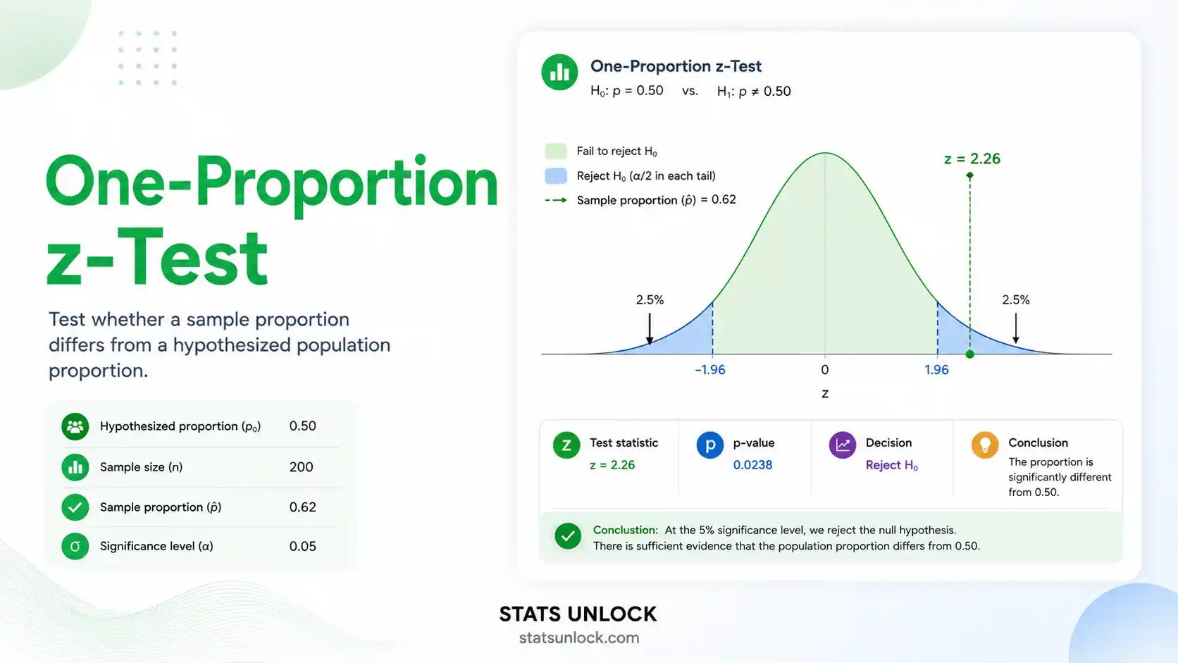
- View the 4 Charts: Chart 1 compares observed vs. expected proportions. Chart 2 shows the z-distribution with rejection regions. Chart 3 shows the confidence interval. Chart 4 shows the outcome frequency breakdown.
- Export: Click "Download Doc" for a plain-text results file, or "Download PDF" to print / save as PDF. Use the five write-up templates to copy APA, thesis, or plain-language result statements.
What is a one-proportion z-test and when should I use it?
A one-proportion z-test checks whether an observed sample proportion differs significantly from a known or hypothesised population proportion. It is used whenever you have a single group with binary (yes/no, pass/fail, infected/healthy) outcomes and a large enough sample. For example, a public health researcher might test whether vaccination coverage in a district (75%) significantly falls short of the national target (80%).
What is a p-value, and how do I interpret it for this test?
The p-value is the probability of observing a proportion as extreme as yours — or more extreme — purely by chance, assuming the null hypothesis is true. It does not mean the probability that the null hypothesis is true. A p-value of 0.03 means: if the true proportion were really p₀, there is only a 3% chance of getting a result this far from p₀. When p < α (your chosen significance level), you reject H₀ and conclude the observed proportion is significantly different.
Does statistical significance mean the difference is practically important?
Not always. With a very large sample, even a tiny difference between p̂ and p₀ can produce a statistically significant result. That does not mean the difference is meaningful in practice. Always report Cohen's h effect size alongside the p-value. A statistically significant result with h = 0.05 might be too small to matter in the real world, while a non-significant result with h = 0.40 might be practically important but require a larger sample to detect reliably.
What is Cohen's h and how do I interpret it?
Cohen's h is the effect size measure for proportion differences. It is calculated by transforming both proportions using the arcsine transformation and taking their difference: h = 2arcsin(√p̂) − 2arcsin(√p₀). Cohen (1988) defined benchmarks: small effect = 0.20, medium effect = 0.50, large effect = 0.80. A negative h means the observed proportion is below p₀; a positive h means it is above. Effect sizes below 0.20 are generally considered trivially small.
What assumptions does the one-proportion z-test require?
The test has four key assumptions: (1) Random sampling — data must come from a random or representative sample; (2) Binary outcomes — each observation must be either a success or failure; (3) Large sample — np₀ ≥ 10 and n(1−p₀) ≥ 10 must both be satisfied for the normal approximation to be valid; (4) Independence — observations must be independent, and the population should be at least 10 times the sample size. If np₀ < 10 or n(1−p₀) < 10, use the exact binomial test instead.
How large a sample do I need for the one-proportion z-test?
The minimum requirement is np₀ ≥ 10 and n(1−p₀) ≥ 10. For statistical power, the sample size depends on the effect you want to detect. To detect a medium effect (h = 0.50) at α = 0.05 with 80% power, you need approximately 33 observations. For a small effect (h = 0.20), you need approximately 197 observations. Very small samples (< 10) should use the exact binomial test, which does not rely on the normal approximation.
What is the difference between one-tailed and two-tailed testing?
A two-tailed test checks whether the proportion differs from p₀ in either direction — higher or lower. A right-tailed test only checks if p̂ > p₀, and a left-tailed test only checks if p̂ < p₀. Two-tailed tests are more conservative (higher p-value) but are the standard choice unless you have a strong, pre-specified directional hypothesis made before data collection. Switching to a one-tailed test after seeing the data inflates your Type I error rate.
How do I report a one-proportion z-test in APA 7th edition format?
Report all required elements: test name, sample proportion, null proportion, z-statistic, p-value, effect size, and confidence interval. Example: "A one-proportion z-test indicated that the observed proportion (p̂ = .63, n = 100) was significantly greater than the hypothesised proportion (p₀ = .50), z = 2.60, p = .009, h = 0.26 (small-to-medium), 95% CI [0.53, 0.72]." See the five auto-filled write-up templates in the Interpretation section for more formats.
Can I use this calculator for published research or a university assignment?
This tool is designed for educational use and exploratory analysis. The calculations follow standard formulas used in peer-reviewed statistics textbooks. For formal research publications, we recommend verifying results using established software such as R (prop.test()), Python (scipy.stats.binom_test()), or SPSS. You can cite this tool as: StatsUnlock. (2025). One-proportion z-test calculator. Retrieved from https://statsunlock.com/one-proportion-z-test-calculator/
What should I do if my result is non-significant?
A non-significant result (p > α) does not prove the null hypothesis is true — it only means your data do not provide sufficient evidence to reject it. This could be due to a genuinely small or absent effect, or because your sample size was too small to detect the effect (low power / Type II error). Report the effect size (Cohen's h) regardless. If h is moderate or large but p is not significant, your study may be underpowered — consider increasing your sample size and collecting more data before drawing conclusions.
📚 References
The one-proportion z-test calculator on this page is based on methods and formulas from the following peer-reviewed sources on proportion hypothesis testing, effect size estimation, and statistical inference.
- Cohen, J. (1988). Statistical power analysis for the behavioral sciences (2nd ed.). Lawrence Erlbaum Associates. https://doi.org/10.4324/9780203771587
- Fleiss, J. L., Levin, B., & Paik, M. C. (2003). Statistical methods for rates and proportions (3rd ed.). John Wiley & Sons. https://doi.org/10.1002/0471445428
- Wilson, E. B. (1927). Probable inference, the law of succession, and statistical inference. Journal of the American Statistical Association, 22(158), 209–212. https://doi.org/10.1080/01621459.1927.10502953
- Newcombe, R. G. (1998). Two-sided confidence intervals for the single proportion: Comparison of seven methods. Statistics in Medicine, 17(8), 857–872. https://doi.org/10.1002/(SICI)1097-0258(19980430)17:8
- Agresti, A., & Coull, B. A. (1998). Approximate is better than "exact" for interval estimation of binomial proportions. The American Statistician, 52(2), 119–126. https://doi.org/10.2307/2685469
- Lakens, D. (2013). Calculating and reporting effect sizes to facilitate cumulative science: A practical primer for t-tests and ANOVAs. Frontiers in Psychology, 4, 863. https://doi.org/10.3389/fpsyg.2013.00863
- Wasserstein, R. L., & Lazar, N. A. (2016). The ASA statement on p-values: Context, process, and purpose. The American Statistician, 70(2), 129–133. https://doi.org/10.1080/00031305.2016.1154108
- Sullivan, G. M., & Feinn, R. (2012). Using effect size — or why the p value is not enough. Journal of Graduate Medical Education, 4(3), 279–282. https://doi.org/10.4300/JGME-D-12-00156.1
- American Psychological Association. (2020). Publication manual of the American Psychological Association (7th ed.). https://doi.org/10.1037/0000165-000
- Pearson, K. (1900). On the criterion that a given system of deviations from the probable in the case of a correlated system of variables is such that it can be reasonably supposed to have arisen from random sampling. Philosophical Magazine, 50(302), 157–175. https://doi.org/10.1080/14786440009463897
- Clopper, C. J., & Pearson, E. S. (1934). The use of confidence or fiducial limits illustrated in the case of the binomial. Biometrika, 26(4), 404–413. https://doi.org/10.2307/2331986
- Cumming, G. (2014). The new statistics: Why and how. Psychological Science, 25(1), 7–29. https://doi.org/10.1177/0956797613504966
- R Core Team. (2024). R: A language and environment for statistical computing. R Foundation for Statistical Computing. https://www.R-project.org/
- Virtanen, P., Gommers, R., Oliphant, T. E., et al. (2020). SciPy 1.0: Fundamental algorithms for scientific computing in Python. Nature Methods, 17, 261–272. https://doi.org/10.1038/s41592-020-0772-5
- Abramowitz, M., & Stegun, I. A. (Eds.). (1964). Handbook of mathematical functions with formulas, graphs, and mathematical tables. National Bureau of Standards. https://doi.org/10.1119/1.15378