


T-Score Calculator
Both meanings of "t-score" in one place. Run a one-sample, two-sample, Welch or paired t-test with degrees of freedom, p-values, confidence intervals and effect sizes. Or convert to the T = 50 + 10z psychometric scale used by the MMPI, BASC and ASEBA, and read a bone-density DXA T-score.
⚡ 0. Quick Answer
A t-score is one of two completely different things, and confusing them is the most common mistake on this topic.
📊 Meaning 1: the t-statistic
An inferential test statistic. It measures how many standard errors a sample mean sits from a hypothesised value.
t = (x̄ − μ) ÷ (s ÷ √n)
It always comes with degrees of freedom, and you convert it to a p-value using the t-distribution. Typical values run from about −4 to +4. This is what you want if you are testing a hypothesis.
🧠 Meaning 2: the T-score scale
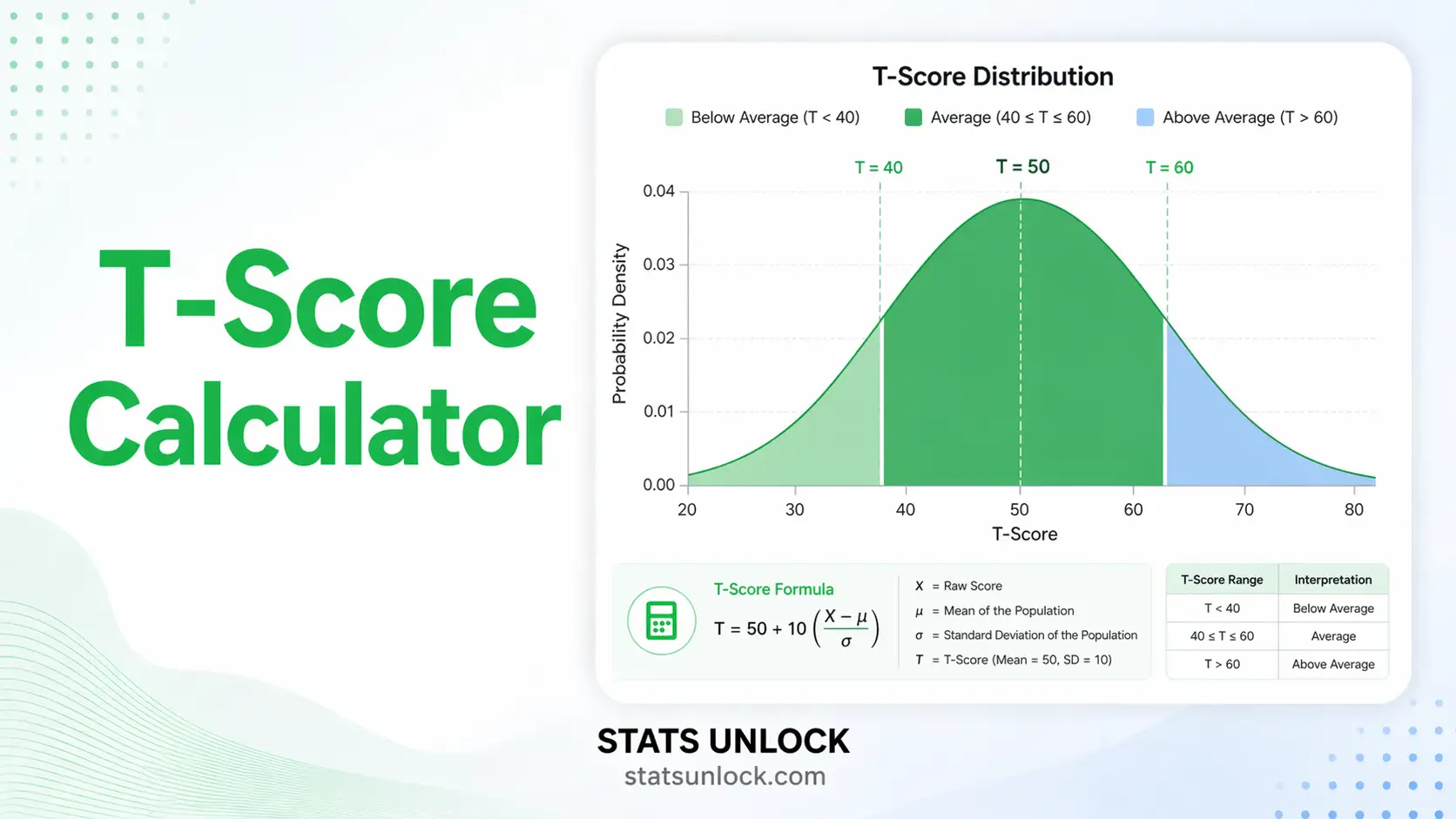
A standardised score scale with a mean of 50 and a standard deviation of 10. It is just a z-score, rescaled to avoid decimals and negative numbers.
T = 50 + 10z
Used in psychometrics (MMPI, BASC, ASEBA, where T above 65 is clinically significant) and, on a different scale entirely, in bone-density DXA scans. Typical values run from 20 to 80.
Key takeaways
- The t-statistic uses the standard error, not the standard deviation. Dividing by s alone is the single most common arithmetic error in a t-test.
- Degrees of freedom drive everything. With df = 4 you need |t| > 2.776 for significance at the 5% level; with df = 100 you only need 1.984, and by df = 1000 it has converged on the normal value of 1.96.
- Use t, not z, whenever you estimated the standard deviation from your data. That is almost always. The t-distribution has heavier tails to account for that extra uncertainty.
- Welch's t-test should be your default for two independent samples. It does not assume equal variances and costs almost nothing when they happen to be equal.
- A p-value is not an effect size. Report Cohen's d and a confidence interval alongside every t-test, because with a large enough sample a trivial difference becomes significant.
- T = 50 + 10z has nothing to do with the t-distribution. They share a letter and nothing else. A T-score of 70 means two standard deviations above the mean, not a test statistic of 70.
📚 1. What Is a T-Score?
1.1 The t-statistic, and why it exists
Suppose you want to know whether a sample mean differs from some hypothesised value. If you knew the population standard deviation you would compute a z-score and read the p-value off the normal curve. In practice you almost never know it, so you estimate it from the same small sample you are testing. That estimate is itself uncertain, and ignoring that uncertainty makes your p-values too small.
William Sealy Gosset worked out the correct distribution in 1908 while employed at the Guinness brewery in Dublin, where he was testing small batches of barley. The brewery would not let staff publish under their own names, so he used the pseudonym "Student", and the distribution has been called Student's t ever since.
The formula looks almost identical to a z-score. The only change is the denominator:
t = (x̄ − μ) ÷ (s ÷ √n)The quantity s ÷ √n is the standard error of the mean. It is smaller than s, because sample means vary far less than individual observations do, and it shrinks as the sample grows.
1.2 Degrees of freedom, in plain terms
Degrees of freedom count how many values in a calculation are genuinely free to vary. Once you have computed a sample mean from n numbers, only n − 1 of those numbers can vary freely: the last one is pinned down by the requirement that they average to the mean you already used. That is why a one-sample t-test has df = n − 1.
Degrees of freedom matter because they set the shape of the distribution. At df = 1 the t-distribution has extraordinarily heavy tails and the 5% critical value is 12.706. At df = 10 it is 2.228. At df = 30 it is 2.042. As df grows the distribution converges on the standard normal, and by df = 1000 the critical value is 1.962, essentially the normal 1.960.
1.3 The four t-tests
| Test | Use when | Degrees of freedom |
|---|---|---|
| One-sample | Comparing one sample mean against a known or hypothesised value | n − 1 |
| Two-sample, Student | Two independent groups, variances assumed equal | n₁ + n₂ − 2 |
| Two-sample, Welch | Two independent groups, variances not assumed equal. The safer default | Welch-Satterthwaite, usually fractional |
| Paired | Two measurements on the same subjects, such as before and after | n pairs − 1 |
1.4 The T-score scale, which is a different animal entirely
The other T-score is not a test statistic at all. It is a linear rescaling of the z-score, chosen so that scores are positive, whole-ish numbers clustered around 50:
T = 50 + 10zA z of 0 becomes T = 50, a z of +1 becomes T = 60, a z of +2 becomes T = 70. Because the transformation is linear, it changes nothing about the data: the percentile attached to T = 70 is exactly the percentile attached to z = 2, which is 97.7%.
Psychological instruments use it heavily. On the MMPI-2, the BASC-3 and the ASEBA family, a T-score of 65 or above (z = 1.5, the 93rd percentile) is conventionally the clinical threshold, with 60 to 64 flagged as at-risk. This convention is why the scale exists: clinicians wanted a single memorable cut-off rather than decimals.
🧮 2. Set Up Your Calculation
Tests whether one sample mean differs from a hypothesised population value. Paste your raw numbers and the calculator works out the mean, standard deviation, standard error and degrees of freedom.
📁 Or upload a CSV / Excel file
Compares the means of two independent groups. Welch's version does not assume the two variances are equal and is the safer default; both are reported side by side so you can see whether the choice matters.
For two measurements on the same subjects, such as before and after a treatment. The test runs on the differences, so the two columns must be the same length and in matching order.
If you only have the published summary statistics and not the raw data, enter them here. This is the usual situation when re-analysing a result from a paper.
The psychometric T-score scale, mean 50 and standard deviation 10. Convert in either direction, and see the percentile plus the clinical band used by instruments such as the MMPI-2, BASC-3 and ASEBA.
Bone mineral density T-score from a DXA scan. This compares your BMD against a healthy young adult reference and uses the WHO diagnostic thresholds. It is not the 50 + 10z scale.
📊 3. Results
🧠 4. Interpretation of Results, In Detail
4.1 What the t-statistic actually measures
A t-statistic is a signal-to-noise ratio. The numerator is the effect you observed, such as how far a sample mean sits from a hypothesised value or how far two group means sit from each other. The denominator is the standard error, which is how much that same quantity would be expected to wobble from sample to sample by chance alone.
So t = 3 means the observed effect is three times larger than the typical chance wobble. t = 0.5 means the effect is smaller than the noise, and you would see something that large routinely even if nothing real were going on. That is the entire logic, and everything else on this page is bookkeeping around it.
4.2 Degrees of freedom, and why the same t means different things
A t of 2.5 is not a fixed amount of evidence. On 3 degrees of freedom it gives p = 0.088 and would not be significant at the 5% level. On 30 degrees of freedom the same 2.5 gives p = 0.018 and would be. On 300 it gives p = 0.013.
The reason is that the t-distribution's shape depends on df. With few degrees of freedom the standard deviation estimate is unreliable, so the distribution has heavy tails to accommodate that, and you need a larger statistic to be convincing. As df grows, the estimate settles down and the distribution converges on the normal curve. Chart 3 in the results plots this convergence directly.
4.3 What a p-value does and does not say
The p-value is the probability of observing a statistic at least this extreme if the null hypothesis were true. That conditional clause carries all the weight. It is not the probability that the null hypothesis is true, it is not the probability that your result is a fluke, and it is not a measure of how large or important the effect is.
A p-value above your alpha does not demonstrate that there is no effect. It means this particular sample was not able to distinguish the effect from zero, which is a statement about your study's power as much as about reality. Absence of evidence is not evidence of absence, and with small samples the two are easily confused.
4.4 Why the confidence interval is the more useful output
A p-value collapses everything into a single yes-or-no verdict. A confidence interval tells you the range of effect sizes the data are compatible with, which is almost always the thing you actually wanted to know.
Two studies can both report p = 0.04, but if one has an interval from 0.1 to 9.8 and the other from 4.2 to 5.6, they are telling you completely different things. The first has established little beyond a direction; the second has pinned the effect down. Reporting the interval also makes non-significant results informative: an interval from −0.2 to 0.3 rules out any large effect, whereas one from −12 to 15 rules out nothing at all.
4.5 Effect size, and why significance is not importance
Statistical significance depends on both the size of the effect and the size of the sample. With 10,000 observations a difference of no practical consequence will be highly significant; with 8 observations a large and important difference may not reach significance at all.
Cohen's d strips out the sample size by expressing the difference in standard deviation units. Cohen's rough conventions are 0.2 for small, 0.5 for medium and 0.8 for large, though he was explicit that these were rules of thumb for fields with no better benchmarks. Where your discipline has its own norms, use those instead. For two-sample tests, Hedges' g applies a small-sample correction to d and is preferable below about n = 20 per group.
4.6 Welch versus Student, and why Welch should be your default
Student's two-sample test assumes both groups have the same population variance and pools them into a single estimate. Welch's test does not, and adjusts the degrees of freedom downwards using the Welch-Satterthwaite equation, which usually produces a fractional value like 15.49.
The evidence favours Welch as a routine default. When the variances really are equal, Welch loses almost nothing. When they are not, particularly with unequal sample sizes, Student's test can have a false positive rate far above the nominal 5%. Both are always computed and displayed side by side in the results table so you can see whether the choice made any difference in your case.
4.7 Paired versus independent, and why the distinction matters so much
If each subject contributes two measurements, the paired test analyses the differences and the between-subject variability cancels out entirely. This usually produces a far smaller standard error and a much more sensitive test.
Applying an independent two-sample test to paired data throws that advantage away and is a genuine statistical error, not merely a conservative choice. The reverse error is worse: pairing observations that are not actually linked manufactures a relationship that is not there. The test to use is determined by how the data were collected, not by which gives the nicer p-value.
4.8 The assumptions, ranked by how much they matter
Independence matters most. If observations are clustered, repeated or autocorrelated, the effective sample size is smaller than n and the p-value will be too small. No amount of sample size fixes this, and nothing in the output will warn you: it has to be handled in the design.
Normality matters least, and less as n grows. The central limit theorem means the sampling distribution of the mean approaches normality even when the raw data do not, so above roughly n = 30 per group the t-test is quite robust. Below about n = 15 it does real work, and a strongly skewed small sample is a genuine problem. Note that for a paired test the assumption applies to the differences, not the raw columns.
Equal variances matter only for Student's version, which is a good reason to use Welch's instead.
4.9 Reading the four charts
Chart 1 draws the t-distribution for your degrees of freedom with the standard normal dashed behind it, so you can see directly how much heavier the tails are at your df. Your statistic is marked and the p-value region shaded. Chart 2 shows the raw observations with group means, which is where you check for skew and stray values. Chart 3 plots the critical value against degrees of freedom, the single clearest picture of why small samples demand larger statistics. Chart 4 shows the confidence interval against the null value, so you can see at a glance whether it crosses.
4.10 The other T-score, and how to tell which you are looking at
If your number is between about 20 and 80 and came from a psychological questionnaire or a school report, it is the T = 50 + 10z scale, not a test statistic. It has no degrees of freedom and no p-value, because it is a position on a scale rather than a hypothesis test.
If your number is between about −4 and +1 and came from a bone density scan, it is the DXA T-score, which is a plain count of standard deviations from a healthy young adult reference with no rescaling.
If your number is roughly between −5 and +5, arrived with a df and a p-value, and came from analysing a sample, it is the t-statistic. The three share a letter and nothing else.
✍ 5. How to Write Your Results in Research
▶ Run the analysis above to auto-fill all five examples with your results.
📌 Key conventions for this style
- Italicise t, p, M, SD, n and d. Degrees of freedom go in parentheses immediately after t.
- Report p to three decimals, or as p < .001. Never write p = .000.
- Drop the leading zero on p and d, because neither can exceed 1 in absolute terms for p.
- Always give the confidence interval and an effect size, not just the p-value.
- State the tail direction and say that it was chosen in advance.
📌 Key conventions for this style
- For use in parentheses mid-sentence, or in a table footnote.
- Still include df, the CI and the effect size. Space is not an excuse to drop them.
- Useful when the same test is reported many times across a results section.
📌 Key conventions for this style
- For an abstract, a press release, or a report to a non-technical audience.
- Never write t, p, df or "significant" in the statistical sense; general readers hear "significant" as "important".
- Give the size of the effect in the original units, which is what people actually care about.
- Be careful not to overstate a non-significant result as proof of no difference.
📌 Key conventions for this style
- Belongs in the methods section, not the results.
- State which t-test variant you used and why, particularly Welch versus Student.
- Say how normality was assessed, and what you would have done if it failed.
- Confirm that alpha and the tail direction were fixed before looking at the data.
📌 Key conventions for this style
- Essential whenever a result is non-significant, because it distinguishes "no effect" from "no power".
- Report the width of the confidence interval, which is the honest measure of precision.
- Avoid post-hoc observed power, which is a deterministic function of the p-value and adds nothing.
- If the study was powered in advance, state the target effect size and the assumptions used.
∑ 6. Formulas Used
t = (x̄₁ − x̄₂) ÷ √[sₚ²(1/n₁ + 1/n₂)] · df = n₁ + n₂ − 2
df = (s₁²/n₁ + s₂²/n₂)² ÷ [ (s₁²/n₁)²/(n₁−1) + (s₂²/n₂)²/(n₂−1) ]
📝 7. How to Use This Calculator
- Decide first which t-score you actually need. If you have a sample and want a p-value, use one of the first four tabs, which run t-tests. If you have a score from a psychological test or a school report, use the T = 50 + 10z tab. If you have a bone density scan, use the DXA tab. These are three unrelated quantities that happen to share a letter.
- Paste your numbers into the data column. One-sample opens first because it is the most common. Enter values comma-separated exactly as the placeholder shows, and set the hypothesised mean you are testing against. The calculator works out the mean, standard deviation, standard error and degrees of freedom for you.
- For two independent groups, use the two-sample tab. Paste each group into its own box. Both Welch and Student results are always computed and shown side by side, so you can see whether the equal-variance assumption changed anything.
- For before-and-after data, use the paired tab. The two columns must be the same length and in matching order, because row 1 in the first column is paired with row 1 in the second. The counter under the boxes warns you if the lengths do not match.
- If you only have published summary statistics, use the fourth tab. Enter the mean, standard deviation and sample size, and it reconstructs the test. This is the usual situation when re-analysing a result from a paper.
- Add clusters to test several groups at once. Each gets its own mean, standard deviation and t against the same hypothesised value. Every column has its own Clear and Remove button, and Remove is disabled on the last remaining column.
- Or upload a CSV or Excel file. Open the upload panel and click the column names you want. Every column you click becomes its own cluster.
- Choose your tail and alpha before you look at the result. Two-tailed asks whether there is any difference; one-tailed commits to a direction and must be decided in advance. Switching afterwards halves your p-value without justification.
- Press Calculate T-Score. Nothing is computed until you do, and changing any input clears the results so you never read stale numbers.
- Read the confidence interval and effect size, not just the p-value. The interval tells you which effect sizes are compatible with your data, and Cohen's d tells you whether the difference matters. A significant p-value with a trivial d usually just means a large sample.
📊 8. How to Run a t-Test in Excel
Excel has a one-call function that does the whole test, plus the building blocks if you want to see the working. Below is the complete workflow in ten steps, each with a picture of what your sheet should look like.
T.TEST for a p-value in one call, T.DIST.2T and T.INV.2T for the distribution, AVERAGE, STDEV.S and SQRT for the components, and CONFIDENCE.T for the interval.Step 1. Lay the two groups out in columns with headers, and reserve a block for the statistics.
Step 2. AVERAGE gives the mean of group 1, 53.5000.
Step 3. STDEV.S divides by n minus 1, which is what a t-test requires. STDEV.P would be wrong here.
Step 4. The standard error, s divided by the square root of n. This is the denominator of t, and forgetting the SQRT is the most common mistake.
Step 5. The one-sample t-statistic against a hypothesised mean of 50, with df = n minus 1 = 9.
Step 6. T.DIST.2T gives the two-tailed p-value directly, 0.1028. It requires a positive t, hence the ABS.
Step 7. T.INV.2T returns the critical value, 2.2622 at df = 9. Since |t| = 1.82 is below it, the result is not significant at 5%.
Step 8. T.TEST does the whole thing in one call. The third argument is the number of tails and the fourth is the type: 1 paired, 2 equal variance, 3 Welch. Use 3 unless you have a reason not to.
Step 9. CONFIDENCE.T returns the margin of error using the t-distribution, 4.3611. Do not use CONFIDENCE.NORM, which assumes you know the population SD.
Step 10. Mean minus and plus the margin gives the 95% confidence interval, 49.14 to 57.86. It contains 50, which is the same conclusion the p-value gave.
The formula cheat sheet
| What you want | Excel formula | Notes |
|---|---|---|
| Mean | =AVERAGE(A2:A11) | Ignores blanks and text |
| Sample SD | =STDEV.S(A2:A11) | Divides by n minus 1. Always this one for a t-test |
| Count | =COUNT(A2:A11) | Counts numbers only, so it matches what AVERAGE used |
| Standard error | =STDEV.S(A2:A11)/SQRT(COUNT(A2:A11)) | The denominator of t |
| One-sample t | =(AVERAGE(A2:A11)-50)/E5 | Replace 50 with your hypothesised mean |
| Degrees of freedom | =COUNT(A2:A11)-1 | For a one-sample or paired test |
| Two-tailed p from t | =T.DIST.2T(ABS(t),df) | Needs a positive t, hence ABS |
| Right-tail p from t | =T.DIST.RT(t,df) | One-tailed, upper |
| Left-tail p from t | =T.DIST(t,df,TRUE) | Cumulative, so this is the lower tail |
| Critical t, two-tailed | =T.INV.2T(0.05,df) | 2.2622 at df = 9 |
| Critical t, one-tailed | =T.INV(0.95,df) | Note this takes the cumulative probability |
| Paired t-test p | =T.TEST(A2:A11,B2:B11,2,1) | Type 1 is paired |
| Two-sample, equal variance | =T.TEST(A2:A11,B2:B11,2,2) | Type 2 is Student's pooled |
| Two-sample, Welch | =T.TEST(A2:A11,B2:B11,2,3) | Type 3. Use this as your default |
| Margin of error | =CONFIDENCE.T(0.05,sd,n) | Uses t, not z |
| Confidence interval | =mean-margin and =mean+margin | Excludes the null value exactly when p < alpha |
| Pooled SD | =SQRT(((n1-1)*s1^2+(n2-1)*s2^2)/(n1+n2-2)) | For Cohen's d on two samples |
| Cohen's d | =(mean1-mean2)/pooledSD | No built-in function exists |
The T = 50 + 10z scale in Excel
| What you want | Excel formula | Result for a raw score of 68, M 50, SD 12 |
|---|---|---|
| Z-score | =STANDARDIZE(68,50,12) | 1.5000 |
| T-score | =50+10*STANDARDIZE(68,50,12) | 65.00 |
| Percentile | =NORM.S.DIST((T-50)/10,TRUE) | 0.9332, so the 93rd percentile |
| Back to z | =(T-50)/10 | 1.5000 |
| T from a percentile | =50+10*NORM.S.INV(0.93) | 64.76 |
| Clinical flag | =IF(T>=65,"Clinical",IF(T>=60,"At-risk","Typical")) | Clinical |
Six mistakes that catch people out
- Using STDEV.P instead of STDEV.S. A t-test is built on a sample estimate. The population version gives a slightly smaller SD, a slightly larger t and a p-value that is too small.
- Forgetting SQRT in the standard error. Dividing by n instead of the square root of n is the most frequent arithmetic error in the whole procedure.
- Passing a negative t to T.DIST.2T. It returns an error. Wrap it in ABS.
- Confusing T.INV with T.INV.2T.
T.INV.2T(0.05,9)gives 2.2622, whileT.INV(0.05,9)gives −1.8331. They answer different questions. - Choosing T.TEST type 2 out of habit. Type 3, Welch, is the safer default and R uses it by default for good reason.
- Using CONFIDENCE.NORM for a small sample. It assumes the population SD is known and gives an interval that is too narrow.
TTEST, TDIST and TINV names. Be careful with legacy TDIST, whose third argument is the number of tails rather than a cumulative flag.📈 9. How to Run a t-Test in R
Base R does all four t-tests with a single function, t.test(), and no packages at all. The script below runs every variant, converts to the T = 50 + 10z scale, and draws one figure. Copy it whole and it will run.
t.test(x, y) defaults to var.equal = FALSE, meaning it runs Welch, not Student. This is a sensible default, but it surprises people who expect the textbook pooled test and then cannot reproduce a result from SPSS. If you need Student's version you must write var.equal = TRUE explicitly.# T-Score Calculator in R (base R, no packages)
# ---- 1. Your data -----------------------------------------------------
g1 <- c(52, 48, 55, 61, 47, 58, 50, 63, 45, 56)
g2 <- c(71, 68, 75, 66, 73, 70, 69, 77, 64, 72)
mu0 <- 50 # hypothesised mean for the one-sample test
alpha <- 0.05
# ---- 2. One-sample t-test ---------------------------------------------
one <- t.test(g1, mu = mu0, conf.level = 1 - alpha)
print(one)
# the same thing by hand, so you can see where every number comes from
n1 <- length(g1)
m1 <- mean(g1)
s1 <- sd(g1) # sd() always divides by n - 1
se1 <- s1 / sqrt(n1)
t1 <- (m1 - mu0) / se1
df1 <- n1 - 1
p1 <- 2 * pt(-abs(t1), df1)
tcrit1 <- qt(1 - alpha/2, df1)
d1 <- (m1 - mu0) / s1 # Cohen's d
# ---- 3. Two-sample t-tests ---------------------------------------------
welch <- t.test(g1, g2) # Welch is the DEFAULT in R
student <- t.test(g1, g2, var.equal = TRUE) # Student's pooled version
n2 <- length(g2); m2 <- mean(g2); s2 <- sd(g2)
sp <- sqrt(((n1-1)*s1^2 + (n2-1)*s2^2) / (n1+n2-2))
d_two <- (m1 - m2) / sp
g_hedges <- d_two * (1 - 3/(4*(n1+n2) - 9))
# ---- 4. Paired t-test ---------------------------------------------------
before <- c(128,135,142,119,151,133,126,147,138,130)
after <- c(121,128,133,115,140,127,122,136,129,124)
paired <- t.test(before, after, paired = TRUE)
# ---- 5. The OTHER t-score: the T = 50 + 10z scale ----------------------
raw <- 68; ref_mean <- 50; ref_sd <- 12
z_scale <- (raw - ref_mean) / ref_sd
T_scale <- 50 + 10 * z_scale
pct <- pnorm(z_scale) * 100
cat(sprintf("ONE-SAMPLE t(%d) = %.4f, p = %.6f, d = %.4f\n", df1, t1, p1, d1))
cat(sprintf(" mean %.4f, SD %.4f, SE %.4f, %d%% CI [%.4f, %.4f]\n",
m1, s1, se1, round((1-alpha)*100), one$conf.int[1], one$conf.int[2]))
cat(sprintf("WELCH t(%.4f) = %.4f, p = %.3e\n",
welch$parameter, welch$statistic, welch$p.value))
cat(sprintf("STUDENT t(%.0f) = %.4f, p = %.3e\n",
student$parameter, student$statistic, student$p.value))
cat(sprintf(" Cohen's d = %.4f, Hedges' g = %.4f\n", d_two, g_hedges))
cat(sprintf("PAIRED t(%.0f) = %.4f, p = %.3e, mean diff %.4f\n",
paired$parameter, paired$statistic, paired$p.value,
mean(before - after)))
cat(sprintf("T-SCALE raw %g -> z = %.4f -> T = %.2f (%.2fth percentile)\n",
raw, z_scale, T_scale, pct))
# ---- 6. One figure ------------------------------------------------------
grid <- seq(-5, 5, length.out = 600)
plot(grid, dt(grid, df1), type = "l", lwd = 2.2, col = "#4338ca", bty = "n",
xlab = "t value", ylab = "density",
main = sprintf("One-Sample t-Test n=%d, mean=%.2f, SD=%.2f, tested against %g",
n1, m1, s1, mu0))
lines(grid, dnorm(grid), lwd = 1.5, lty = 2, col = "#94a3b8")
# shade both tails beyond |t|
tail_r <- grid[grid >= abs(t1)]
tail_l <- grid[grid <= -abs(t1)]
polygon(c(tail_r, rev(tail_r)), c(dt(tail_r, df1), rep(0, length(tail_r))),
col = adjustcolor("#f59e0b", 0.40), border = NA)
polygon(c(tail_l, rev(tail_l)), c(dt(tail_l, df1), rep(0, length(tail_l))),
col = adjustcolor("#f59e0b", 0.40), border = NA)
abline(v = t1, col = "#be185d", lwd = 2.4)
abline(v = c(-tcrit1, tcrit1), col = "#b45309", lty = 3, lwd = 1.4)
text(tcrit1, max(dt(grid, df1)) * 0.92,
sprintf(" critical %.3f", tcrit1), pos = 4, cex = 0.8, col = "#b45309")
legend("topright", bty = "n", cex = 0.85,
legend = c(sprintf("t-distribution, df = %d", df1),
"normal for comparison",
sprintf("p = %.4f", p1),
sprintf("observed t = %.3f", t1)),
col = c("#4338ca", "#94a3b8", "#f59e0b", "#be185d"),
lwd = c(2.2, 1.5, 6, 2.4), lty = c(1, 2, 1, 1))
What the script prints
ONE-SAMPLE  t(9) = 1.8155, p = 0.102838, d = 0.5741
            mean 53.5000, SD 6.0964, SE 1.9279, 95% CI [49.1389, 57.8611]
WELCH       t(15.4903) = -7.3843, p = 1.876e-06
STUDENT     t(18) = -7.3843, p = 7.519e-07
            Cohen's d = -3.3024, Hedges' g = -3.1628
PAIRED      t(9) = 9.1864, p = 7.217e-06, mean diff 7.4000
T-SCALE     raw 68 -> z = 1.5000 -> T = 65.00 (93.32th percentile)
These are the same numbers the Python script produces and the same numbers the calculator at the top of this page produces, which is a useful sanity check whenever you port an analysis between tools.
Line-by-line explanation
- Block 1 holds the only things you change. Everything below is generic.
- Block 2 runs the one-sample test twice: once with
t.test()and once by hand. The manual version exists so you can see thatpt()is the t-distribution's CDF andqt()its inverse, exactly parallel topnorm()andqnorm()for the normal. - Block 3 shows the Welch and Student versions side by side. Notice that t is identical in this case, at −7.3843, but the degrees of freedom differ (15.49 versus 18) and therefore so do the p-values. When sample sizes are equal, only the df changes; when they are unequal, t changes too.
- Block 4 runs the paired test.
paired = TRUEmakes R analyse the differences, which is not the same as passing the differences to a one-sample test only in that R handles the bookkeeping for you. - Block 5 is the completely unrelated T-score scale, included so the two never get confused. It uses
pnorm(), the normal CDF, not the t-distribution. - Block 6 draws one figure containing everything: the t-distribution for your df, the normal dashed behind it so the heavier tails are visible, the shaded p-value region, your observed t and the critical values.
Useful one-liners
| Task | R |
|---|---|
| One-sample t-test | t.test(x, mu = 50) |
| Two-sample, Welch (default) | t.test(x, y) |
| Two-sample, Student | t.test(x, y, var.equal = TRUE) |
| Paired | t.test(x, y, paired = TRUE) |
| One-tailed | t.test(x, mu = 50, alternative = "greater") |
| Formula interface | t.test(value ~ group, data = df) |
| 99% confidence interval | t.test(x, conf.level = 0.99) |
| Extract just the p-value | t.test(x, y)$p.value |
| Extract the CI | t.test(x, y)$conf.int |
| p from t | 2 * pt(-abs(t), df) |
| Critical t | qt(0.975, df) |
| Check normality | shapiro.test(x) |
| Non-parametric alternative | wilcox.test(x, y) |
| Cohen's d (effsize package) | effsize::cohen.d(x, y) |
| Power analysis (pwr package) | pwr::pwr.t.test(d = 0.5, power = 0.8) |
| T = 50 + 10z | 50 + 10 * scale(x) |
🐍 10. How to Run a t-Test in Python
SciPy has one function per test and returns the statistic, the p-value and the degrees of freedom. The script below was run before being published, so the printed output shown underneath is real, not typed by hand.
np.std() defaults to ddof=0, the population divisor, so you must write ddof=1 whenever you compute a standard deviation by hand for a t-test. Second, scipy.stats.ttest_ind defaults to equal_var=True, which is Student's test. R defaults to Welch. That single difference is why the same data can give two different p-values in the two languages.# T-Score Calculator in Python
# Runs one-sample, two-sample (Welch and Student) and paired t-tests,
# converts to the T = 50 + 10z scale, and draws one summary figure.
import numpy as np
import matplotlib.pyplot as plt
from scipy import stats
# ---- 1. Your data -----------------------------------------------------
g1 = np.array([52, 48, 55, 61, 47, 58, 50, 63, 45, 56], dtype=float)
g2 = np.array([71, 68, 75, 66, 73, 70, 69, 77, 64, 72], dtype=float)
mu0 = 50.0 # hypothesised mean for the one-sample test
alpha = 0.05
# ---- 2. One-sample t-test ---------------------------------------------
n1 = g1.size
m1 = g1.mean()
s1 = g1.std(ddof=1) # ddof=1 is essential: sample SD
se1 = s1 / np.sqrt(n1)
t1 = (m1 - mu0) / se1
df1 = n1 - 1
p1 = 2 * stats.t.sf(abs(t1), df1)
tcrit1 = stats.t.ppf(1 - alpha/2, df1)
ci1 = (m1 - tcrit1*se1, m1 + tcrit1*se1)
d1 = (m1 - mu0) / s1 # Cohen's d
# ---- 3. Two-sample t-tests --------------------------------------------
welch = stats.ttest_ind(g1, g2, equal_var=False)
student = stats.ttest_ind(g1, g2, equal_var=True)
n2, m2, s2 = g2.size, g2.mean(), g2.std(ddof=1)
sp = np.sqrt(((n1-1)*s1**2 + (n2-1)*s2**2) / (n1+n2-2))
d_two = (m1 - m2) / sp
g_hedges = d_two * (1 - 3/(4*(n1+n2) - 9))
# ---- 4. Paired t-test --------------------------------------------------
before = np.array([128,135,142,119,151,133,126,147,138,130], dtype=float)
after = np.array([121,128,133,115,140,127,122,136,129,124], dtype=float)
paired = stats.ttest_rel(before, after)
diffs = before - after
# ---- 5. The OTHER t-score: the T = 50 + 10z scale ---------------------
raw, ref_mean, ref_sd = 68.0, 50.0, 12.0
z_scale = (raw - ref_mean) / ref_sd
T_scale = 50 + 10*z_scale
pct = stats.norm.cdf(z_scale) * 100
print(f"ONE-SAMPLE t({df1}) = {t1:.4f}, p = {p1:.6f}, d = {d1:.4f}")
print(f" mean {m1:.4f}, SD {s1:.4f}, SE {se1:.4f}, "
f"{int((1-alpha)*100)}% CI [{ci1[0]:.4f}, {ci1[1]:.4f}]")
print(f"WELCH t({welch.df:.4f}) = {welch.statistic:.4f}, p = {welch.pvalue:.3e}")
print(f"STUDENT t({student.df:.0f}) = {student.statistic:.4f}, p = {student.pvalue:.3e}")
print(f" Cohen's d = {d_two:.4f}, Hedges' g = {g_hedges:.4f}")
print(f"PAIRED t({paired.df}) = {paired.statistic:.4f}, p = {paired.pvalue:.3e}, "
f"mean diff {diffs.mean():.4f}")
print(f"T-SCALE raw {raw:g} -> z = {z_scale:.4f} -> T = {T_scale:.2f} "
f"({pct:.2f}th percentile)")
# ---- 6. One figure -----------------------------------------------------
fig, ax = plt.subplots(figsize=(9, 5))
grid = np.linspace(-5, 5, 600)
ax.plot(grid, stats.t.pdf(grid, df1), color="#4338ca", lw=2.2,
label=f"t-distribution, df = {df1}")
ax.plot(grid, stats.norm.pdf(grid), color="#94a3b8", lw=1.5, ls="--",
label="normal for comparison")
ax.fill_between(grid, stats.t.pdf(grid, df1), where=np.abs(grid) >= abs(t1),
color="#f59e0b", alpha=.40, label=f"p = {p1:.4f}")
ax.axvline(t1, color="#be185d", lw=2.4, label=f"observed t = {t1:.3f}")
for c in (-tcrit1, tcrit1):
ax.axvline(c, color="#b45309", ls=":", lw=1.4)
ax.text(tcrit1, ax.get_ylim()[1]*.92, f" critical {tcrit1:.3f}",
fontsize=9, color="#b45309")
ax.set_xlabel("t value")
ax.set_ylabel("density")
ax.set_title(f"One-Sample t-Test n={n1}, mean={m1:.2f}, SD={s1:.2f}, "
f"tested against {mu0:g}")
ax.legend(frameon=False, fontsize=9)
ax.spines[["top", "right"]].set_visible(False)
fig.tight_layout()
fig.savefig("t_test_summary.png", dpi=150)
plt.show()
Actual output from running the script
ONE-SAMPLE  t(9) = 1.8155, p = 0.102838, d = 0.5741
            mean 53.5000, SD 6.0964, SE 1.9279, 95% CI [49.1389, 57.8611]
WELCH       t(15.4903) = -7.3843, p = 1.876e-06
STUDENT     t(18) = -7.3843, p = 7.519e-07
            Cohen's d = -3.3024, Hedges' g = -3.1628
PAIRED      t(9) = 9.1864, p = 7.217e-06, mean diff 7.4000
T-SCALE     raw 68 -> z = 1.5000 -> T = 65.00 (93.32th percentile)
Line-by-line explanation
- Block 1 is the only part you edit. Setting
dtype=floatavoids integer surprises later. - Block 2 computes the one-sample test from first principles rather than calling
ttest_1samp, so every intermediate quantity is visible.stats.t.sfis the survival function, which is1 - cdfcomputed accurately in the far tail, and doubling it gives the two-tailed p-value. - Block 3 runs both two-sample variants. Note that
welch.dfis 15.4903, a fractional value produced by the Welch-Satterthwaite equation, while Student's is a whole 18. Hedges' g applies the small-sample correction to Cohen's d, and here it pulls the estimate from −3.3024 down to −3.1628. - Block 4 runs the paired test with
ttest_rel. The name means "related samples". Passing paired data tottest_indinstead would be a genuine error, not a conservative choice. - Block 5 handles the unrelated T = 50 + 10z scale, which uses the normal distribution rather than the t-distribution. It is included here purely so the two never get mixed up.
- Block 6 draws a single figure with the t-distribution, the normal dashed behind it so the heavier tails are visible, the shaded p-value region, the observed t and the critical values.
Useful one-liners
| Task | Python |
|---|---|
| One-sample t-test | stats.ttest_1samp(x, 50) |
| Two-sample, Welch | stats.ttest_ind(x, y, equal_var=False) |
| Two-sample, Student (the default) | stats.ttest_ind(x, y) |
| Paired | stats.ttest_rel(x, y) |
| One-tailed | stats.ttest_ind(x, y, alternative='greater') |
| From summary statistics only | stats.ttest_ind_from_stats(m1,s1,n1,m2,s2,n2) |
| Confidence interval (SciPy 1.10+) | stats.ttest_1samp(x,50).confidence_interval() |
| p from t | 2 * stats.t.sf(abs(t), df) |
| Critical t | stats.t.ppf(0.975, df) |
| Sample SD | x.std(ddof=1) |
| Check normality | stats.shapiro(x) |
| Non-parametric alternatives | stats.mannwhitneyu(x,y), stats.wilcoxon(x,y) |
| Power analysis | statsmodels.stats.power.TTestIndPower().solve_power(...) |
| Pandas group comparison | stats.ttest_ind(*[g.values for _,g in df.groupby('grp')['v']]) |
| T = 50 + 10z | 50 + 10*stats.zscore(x, ddof=1) |
equal_var first. It accounts for the overwhelming majority of such discrepancies, and the difference is entirely in the degrees of freedom.📋 11. Reference Tables
11.1 Critical values of t, two-tailed
Find your degrees of freedom down the left, then read across to your alpha. If your |t| exceeds the value in the cell, the result is significant at that level. The bottom row is the normal distribution, which is where t converges as df grows.
| df | 0.2 | 0.1 | 0.05 | 0.02 | 0.01 | 0.002 | 0.001 |
|---|---|---|---|---|---|---|---|
| 1 | 3.0777 | 6.3138 | 12.7062 | 31.8205 | 63.6567 | 318.309 | 636.619 |
| 2 | 1.8856 | 2.9200 | 4.3027 | 6.9646 | 9.9248 | 22.3271 | 31.5991 |
| 3 | 1.6377 | 2.3534 | 3.1824 | 4.5407 | 5.8409 | 10.2145 | 12.9240 |
| 4 | 1.5332 | 2.1318 | 2.7764 | 3.7469 | 4.6041 | 7.1732 | 8.6103 |
| 5 | 1.4759 | 2.0150 | 2.5706 | 3.3649 | 4.0321 | 5.8934 | 6.8688 |
| 6 | 1.4398 | 1.9432 | 2.4469 | 3.1427 | 3.7074 | 5.2076 | 5.9588 |
| 7 | 1.4149 | 1.8946 | 2.3646 | 2.9980 | 3.4995 | 4.7853 | 5.4079 |
| 8 | 1.3968 | 1.8595 | 2.3060 | 2.8965 | 3.3554 | 4.5008 | 5.0413 |
| 9 | 1.3830 | 1.8331 | 2.2622 | 2.8214 | 3.2498 | 4.2968 | 4.7809 |
| 10 | 1.3722 | 1.8125 | 2.2281 | 2.7638 | 3.1693 | 4.1437 | 4.5869 |
| 11 | 1.3634 | 1.7959 | 2.2010 | 2.7181 | 3.1058 | 4.0247 | 4.4370 |
| 12 | 1.3562 | 1.7823 | 2.1788 | 2.6810 | 3.0545 | 3.9296 | 4.3178 |
| 13 | 1.3502 | 1.7709 | 2.1604 | 2.6503 | 3.0123 | 3.8520 | 4.2208 |
| 14 | 1.3450 | 1.7613 | 2.1448 | 2.6245 | 2.9768 | 3.7874 | 4.1405 |
| 15 | 1.3406 | 1.7531 | 2.1314 | 2.6025 | 2.9467 | 3.7328 | 4.0728 |
| 16 | 1.3368 | 1.7459 | 2.1199 | 2.5835 | 2.9208 | 3.6862 | 4.0150 |
| 17 | 1.3334 | 1.7396 | 2.1098 | 2.5669 | 2.8982 | 3.6458 | 3.9651 |
| 18 | 1.3304 | 1.7341 | 2.1009 | 2.5524 | 2.8784 | 3.6105 | 3.9216 |
| 19 | 1.3277 | 1.7291 | 2.0930 | 2.5395 | 2.8609 | 3.5794 | 3.8834 |
| 20 | 1.3253 | 1.7247 | 2.0860 | 2.5280 | 2.8453 | 3.5518 | 3.8495 |
| 21 | 1.3232 | 1.7207 | 2.0796 | 2.5176 | 2.8314 | 3.5272 | 3.8193 |
| 22 | 1.3212 | 1.7171 | 2.0739 | 2.5083 | 2.8188 | 3.5050 | 3.7921 |
| 23 | 1.3195 | 1.7139 | 2.0687 | 2.4999 | 2.8073 | 3.4850 | 3.7676 |
| 24 | 1.3178 | 1.7109 | 2.0639 | 2.4922 | 2.7969 | 3.4668 | 3.7454 |
| 25 | 1.3163 | 1.7081 | 2.0595 | 2.4851 | 2.7874 | 3.4502 | 3.7251 |
| 26 | 1.3150 | 1.7056 | 2.0555 | 2.4786 | 2.7787 | 3.4350 | 3.7066 |
| 27 | 1.3137 | 1.7033 | 2.0518 | 2.4727 | 2.7707 | 3.4210 | 3.6896 |
| 28 | 1.3125 | 1.7011 | 2.0484 | 2.4671 | 2.7633 | 3.4082 | 3.6739 |
| 29 | 1.3114 | 1.6991 | 2.0452 | 2.4620 | 2.7564 | 3.3962 | 3.6594 |
| 30 | 1.3104 | 1.6973 | 2.0423 | 2.4573 | 2.7500 | 3.3852 | 3.6460 |
| 35 | 1.3062 | 1.6896 | 2.0301 | 2.4377 | 2.7238 | 3.3400 | 3.5911 |
| 40 | 1.3031 | 1.6839 | 2.0211 | 2.4233 | 2.7045 | 3.3069 | 3.5510 |
| 45 | 1.3006 | 1.6794 | 2.0141 | 2.4121 | 2.6896 | 3.2815 | 3.5203 |
| 50 | 1.2987 | 1.6759 | 2.0086 | 2.4033 | 2.6778 | 3.2614 | 3.4960 |
| 60 | 1.2958 | 1.6706 | 2.0003 | 2.3901 | 2.6603 | 3.2317 | 3.4602 |
| 70 | 1.2938 | 1.6669 | 1.9944 | 2.3808 | 2.6479 | 3.2108 | 3.4350 |
| 80 | 1.2922 | 1.6641 | 1.9901 | 2.3739 | 2.6387 | 3.1953 | 3.4163 |
| 90 | 1.2910 | 1.6620 | 1.9867 | 2.3685 | 2.6316 | 3.1833 | 3.4019 |
| 100 | 1.2901 | 1.6602 | 1.9840 | 2.3642 | 2.6259 | 3.1737 | 3.3905 |
| 120 | 1.2886 | 1.6577 | 1.9799 | 2.3578 | 2.6174 | 3.1595 | 3.3735 |
| 150 | 1.2872 | 1.6551 | 1.9759 | 2.3515 | 2.6090 | 3.1455 | 3.3566 |
| 200 | 1.2858 | 1.6525 | 1.9719 | 2.3451 | 2.6006 | 3.1315 | 3.3398 |
| 300 | 1.2844 | 1.6499 | 1.9679 | 2.3388 | 2.5923 | 3.1176 | 3.3233 |
| 500 | 1.2832 | 1.6479 | 1.9647 | 2.3338 | 2.5857 | 3.1066 | 3.3101 |
| 1000 | 1.2824 | 1.6464 | 1.9623 | 2.3301 | 2.5808 | 3.0984 | 3.3003 |
| ∞ (z) | 1.2816 | 1.6449 | 1.9600 | 2.3263 | 2.5758 | 3.0902 | 3.2905 |
11.2 Critical values of t, one-tailed
Same table for a directional hypothesis. Note that the one-tailed value at alpha 0.025 equals the two-tailed value at alpha 0.05, which is the arithmetic behind the warning about switching tails after seeing your data.
| df | 0.1 | 0.05 | 0.025 | 0.01 | 0.005 | 0.001 | 0.0005 |
|---|---|---|---|---|---|---|---|
| 1 | 3.0777 | 6.3138 | 12.7062 | 31.8205 | 63.6567 | 318.309 | 636.619 |
| 2 | 1.8856 | 2.9200 | 4.3027 | 6.9646 | 9.9248 | 22.3271 | 31.5991 |
| 3 | 1.6377 | 2.3534 | 3.1824 | 4.5407 | 5.8409 | 10.2145 | 12.9240 |
| 4 | 1.5332 | 2.1318 | 2.7764 | 3.7469 | 4.6041 | 7.1732 | 8.6103 |
| 5 | 1.4759 | 2.0150 | 2.5706 | 3.3649 | 4.0321 | 5.8934 | 6.8688 |
| 6 | 1.4398 | 1.9432 | 2.4469 | 3.1427 | 3.7074 | 5.2076 | 5.9588 |
| 7 | 1.4149 | 1.8946 | 2.3646 | 2.9980 | 3.4995 | 4.7853 | 5.4079 |
| 8 | 1.3968 | 1.8595 | 2.3060 | 2.8965 | 3.3554 | 4.5008 | 5.0413 |
| 9 | 1.3830 | 1.8331 | 2.2622 | 2.8214 | 3.2498 | 4.2968 | 4.7809 |
| 10 | 1.3722 | 1.8125 | 2.2281 | 2.7638 | 3.1693 | 4.1437 | 4.5869 |
| 11 | 1.3634 | 1.7959 | 2.2010 | 2.7181 | 3.1058 | 4.0247 | 4.4370 |
| 12 | 1.3562 | 1.7823 | 2.1788 | 2.6810 | 3.0545 | 3.9296 | 4.3178 |
| 13 | 1.3502 | 1.7709 | 2.1604 | 2.6503 | 3.0123 | 3.8520 | 4.2208 |
| 14 | 1.3450 | 1.7613 | 2.1448 | 2.6245 | 2.9768 | 3.7874 | 4.1405 |
| 15 | 1.3406 | 1.7531 | 2.1314 | 2.6025 | 2.9467 | 3.7328 | 4.0728 |
| 16 | 1.3368 | 1.7459 | 2.1199 | 2.5835 | 2.9208 | 3.6862 | 4.0150 |
| 17 | 1.3334 | 1.7396 | 2.1098 | 2.5669 | 2.8982 | 3.6458 | 3.9651 |
| 18 | 1.3304 | 1.7341 | 2.1009 | 2.5524 | 2.8784 | 3.6105 | 3.9216 |
| 19 | 1.3277 | 1.7291 | 2.0930 | 2.5395 | 2.8609 | 3.5794 | 3.8834 |
| 20 | 1.3253 | 1.7247 | 2.0860 | 2.5280 | 2.8453 | 3.5518 | 3.8495 |
| 21 | 1.3232 | 1.7207 | 2.0796 | 2.5176 | 2.8314 | 3.5272 | 3.8193 |
| 22 | 1.3212 | 1.7171 | 2.0739 | 2.5083 | 2.8188 | 3.5050 | 3.7921 |
| 23 | 1.3195 | 1.7139 | 2.0687 | 2.4999 | 2.8073 | 3.4850 | 3.7676 |
| 24 | 1.3178 | 1.7109 | 2.0639 | 2.4922 | 2.7969 | 3.4668 | 3.7454 |
| 25 | 1.3163 | 1.7081 | 2.0595 | 2.4851 | 2.7874 | 3.4502 | 3.7251 |
| 26 | 1.3150 | 1.7056 | 2.0555 | 2.4786 | 2.7787 | 3.4350 | 3.7066 |
| 27 | 1.3137 | 1.7033 | 2.0518 | 2.4727 | 2.7707 | 3.4210 | 3.6896 |
| 28 | 1.3125 | 1.7011 | 2.0484 | 2.4671 | 2.7633 | 3.4082 | 3.6739 |
| 29 | 1.3114 | 1.6991 | 2.0452 | 2.4620 | 2.7564 | 3.3962 | 3.6594 |
| 30 | 1.3104 | 1.6973 | 2.0423 | 2.4573 | 2.7500 | 3.3852 | 3.6460 |
| 35 | 1.3062 | 1.6896 | 2.0301 | 2.4377 | 2.7238 | 3.3400 | 3.5911 |
| 40 | 1.3031 | 1.6839 | 2.0211 | 2.4233 | 2.7045 | 3.3069 | 3.5510 |
| 45 | 1.3006 | 1.6794 | 2.0141 | 2.4121 | 2.6896 | 3.2815 | 3.5203 |
| 50 | 1.2987 | 1.6759 | 2.0086 | 2.4033 | 2.6778 | 3.2614 | 3.4960 |
| 60 | 1.2958 | 1.6706 | 2.0003 | 2.3901 | 2.6603 | 3.2317 | 3.4602 |
| 70 | 1.2938 | 1.6669 | 1.9944 | 2.3808 | 2.6479 | 3.2108 | 3.4350 |
| 80 | 1.2922 | 1.6641 | 1.9901 | 2.3739 | 2.6387 | 3.1953 | 3.4163 |
| 90 | 1.2910 | 1.6620 | 1.9867 | 2.3685 | 2.6316 | 3.1833 | 3.4019 |
| 100 | 1.2901 | 1.6602 | 1.9840 | 2.3642 | 2.6259 | 3.1737 | 3.3905 |
| 120 | 1.2886 | 1.6577 | 1.9799 | 2.3578 | 2.6174 | 3.1595 | 3.3735 |
| 150 | 1.2872 | 1.6551 | 1.9759 | 2.3515 | 2.6090 | 3.1455 | 3.3566 |
| 200 | 1.2858 | 1.6525 | 1.9719 | 2.3451 | 2.6006 | 3.1315 | 3.3398 |
| 300 | 1.2844 | 1.6499 | 1.9679 | 2.3388 | 2.5923 | 3.1176 | 3.3233 |
| 500 | 1.2832 | 1.6479 | 1.9647 | 2.3338 | 2.5857 | 3.1066 | 3.3101 |
| 1000 | 1.2824 | 1.6464 | 1.9623 | 2.3301 | 2.5808 | 3.0984 | 3.3003 |
| ∞ (z) | 1.2816 | 1.6449 | 1.9600 | 2.3263 | 2.5758 | 3.0902 | 3.2905 |
11.3 How fast t converges on z
This is the table that answers "when can I just use z?". The difference is 15% at df = 5, under 3% by df = 30, and under 1% by df = 100. There is never a penalty for using t, so the honest answer is: always use t when you estimated the standard deviation.
| df | Critical t (5%, two-tailed) | Critical z | Difference | Relative |
|---|---|---|---|---|
| 1 | 12.7062 | 1.9600 | +10.7462 | +548.29% |
| 2 | 4.3027 | 1.9600 | +2.3427 | +119.53% |
| 3 | 3.1824 | 1.9600 | +1.2225 | +62.37% |
| 5 | 2.5706 | 1.9600 | +0.6106 | +31.15% |
| 10 | 2.2281 | 1.9600 | +0.2682 | +13.68% |
| 15 | 2.1314 | 1.9600 | +0.1715 | +8.75% |
| 20 | 2.0860 | 1.9600 | +0.1260 | +6.43% |
| 25 | 2.0595 | 1.9600 | +0.0996 | +5.08% |
| 30 | 2.0423 | 1.9600 | +0.0823 | +4.20% |
| 40 | 2.0211 | 1.9600 | +0.0611 | +3.12% |
| 50 | 2.0086 | 1.9600 | +0.0486 | +2.48% |
| 60 | 2.0003 | 1.9600 | +0.0403 | +2.06% |
| 100 | 1.9840 | 1.9600 | +0.0240 | +1.22% |
| 200 | 1.9719 | 1.9600 | +0.0119 | +0.61% |
| 500 | 1.9647 | 1.9600 | +0.0048 | +0.24% |
| 1000 | 1.9623 | 1.9600 | +0.0024 | +0.12% |
11.4 The same t gives very different p-values
Read across any row to see how much the degrees of freedom matter. A t of 2.5 is not significant at df = 3 (p = 0.088) but is at df = 20 (p = 0.021). This is why reporting t without df is meaningless.
| |t| | df 3 | df 5 | df 10 | df 20 | df 30 | df 60 | df 120 | z (df ∞) |
|---|---|---|---|---|---|---|---|---|
| 1.0 | 0.3910 | 0.3632 | 0.3409 | 0.3293 | 0.3253 | 0.3213 | 0.3193 | 0.3173 |
| 1.5 | 0.2306 | 0.1939 | 0.1645 | 0.1492 | 0.1441 | 0.1389 | 0.1362 | 0.1336 |
| 2.0 | 0.1393 | 0.1019 | 0.0734 | 0.0593 | 0.0546 | 0.0500 | 0.0478 | 0.0455 |
| 2.5 | 0.0877 | 0.0545 | 0.0314 | 0.0212 | 0.0181 | 0.0152 | 0.0138 | 0.0124 |
| 3.0 | 0.0577 | 0.0301 | 0.0133 | 0.0071 | 0.0054 | 0.0039 | 0.0033 | 0.0027 |
| 3.5 | 0.0395 | 0.0173 | 0.0057 | 0.0023 | 0.0015 | 0.0009 | 0.0007 | 0.0005 |
11.5 The T = 50 + 10z scale, full conversion table
Every standardised score system in this table is the same z-score wearing different clothes. The clinical bands are the conventions used across the MMPI, BASC and ASEBA families; your specific test manual takes precedence.
| T-score | z | Percentile | IQ scale M 100, SD 15 | Scaled M 10, SD 3 | Stanine | Sten | NCE | Typical clinical band |
|---|---|---|---|---|---|---|---|---|
| 20 | -3.0 | 0.13 | 55.0 | 1.0 | 1 | 1 | -13.2 | Low |
| 25 | -2.5 | 0.62 | 62.5 | 2.5 | 1 | 1 | -2.6 | Low |
| 30 | -2.0 | 2.28 | 70.0 | 4.0 | 1 | 2 | 7.9 | Low |
| 35 | -1.5 | 6.68 | 77.5 | 5.5 | 2 | 2 | 18.4 | Low |
| 40 | -1.0 | 15.87 | 85.0 | 7.0 | 3 | 4 | 28.9 | Low |
| 45 | -0.5 | 30.85 | 92.5 | 8.5 | 4 | 4 | 39.5 | Average |
| 50 | +0.0 | 50.00 | 100.0 | 10.0 | 5 | 6 | 50.0 | Average |
| 55 | +0.5 | 69.15 | 107.5 | 11.5 | 6 | 6 | 60.5 | Average |
| 60 | +1.0 | 84.13 | 115.0 | 13.0 | 7 | 8 | 71.1 | At-risk / elevated |
| 65 | +1.5 | 93.32 | 122.5 | 14.5 | 8 | 8 | 81.6 | Clinically significant |
| 70 | +2.0 | 97.72 | 130.0 | 16.0 | 9 | 10 | 92.1 | Clinically significant, marked |
| 75 | +2.5 | 99.38 | 137.5 | 17.5 | 9 | 10 | 102.7 | Clinically significant, marked |
| 80 | +3.0 | 99.87 | 145.0 | 19.0 | 9 | 10 | 113.2 | Clinically significant, marked |
| 85 | +3.5 | 99.98 | 152.5 | 20.5 | 9 | 10 | 123.7 | Clinically significant, marked |
Conversion formulas: z = (T − 50) ÷ 10, IQ = 100 + 15z, Wechsler scaled = 10 + 3z, stanine = 5 + 2z rounded and clipped to 1-9, sten = 5.5 + 2z rounded and clipped to 1-10, NCE = 50 + 21.06z.
11.6 Statistical power and the sample size you need
Power is the probability of detecting an effect that is really there. The right-hand column is the number you should look at before collecting data, not after. These figures are for a two-sample test at alpha 0.05, two-tailed.
| Cohen's d | n=10 per group | n=20 | n=30 | n=50 | n=100 | n=200 | n needed for 80% power |
|---|---|---|---|---|---|---|---|
| 0.2 | 7.1% | 9.5% | 11.9% | 16.8% | 29.1% | 51.4% | 394 |
| 0.5 | 18.5% | 33.8% | 47.8% | 69.7% | 94.0% | 99.9% | 7470 |
| 0.8 | 39.5% | 69.3% | 86.1% | 97.7% | 100.0% | 100.0% | 2107 |
| 1.0 | 56.2% | 86.9% | 96.8% | 99.9% | 100.0% | nan% | 2643 |
| 1.2 | 71.8% | 95.9% | 99.5% | 100.0% | 100.0% | nan% | 1250 |
11.7 Bone density T-score thresholds (WHO)
| T-score | WHO category | Percentile of young adults | Typical interpretation |
|---|---|---|---|
| ≥ −1.0 | Normal | 16th and above | Bone density within the expected range for a healthy young adult |
| −1.0 to −2.5 | Osteopenia (low bone mass) | 1st to 16th | Below normal but not osteoporosis. Monitoring and lifestyle measures usually discussed |
| ≤ −2.5 | Osteoporosis | Below the 1st | Meets the WHO diagnostic definition |
| ≤ −2.5 with a fracture | Severe / established osteoporosis | Below the 1st | Osteoporosis plus one or more fragility fractures |
Defined for the lumbar spine, total hip and femoral neck. The Z-score, which compares against age-matched and sex-matched peers rather than young adults, is used instead for premenopausal women, men under 50 and children, where a Z below −2.0 prompts investigation for secondary causes.
11.8 Which test do you actually need?
| Your situation | Test | Degrees of freedom | Non-parametric alternative |
|---|---|---|---|
| One sample against a known value | One-sample t-test | n − 1 | Wilcoxon signed-rank |
| Two independent groups | Welch's t-test | Welch-Satterthwaite | Mann-Whitney U |
| Two independent groups, equal variances known | Student's t-test | n₁ + n₂ − 2 | Mann-Whitney U |
| Before and after on the same subjects | Paired t-test | pairs − 1 | Wilcoxon signed-rank |
| Three or more groups | One-way ANOVA | k−1 and N−k | Kruskal-Wallis |
| Population SD genuinely known | z-test | none | - |
| Proportions rather than means | Chi-square or a proportions test | varies | Fisher's exact |
| A score against published norms | Not a test. Use the T = 50 + 10z scale | none | - |
11.9 Effect size benchmarks
| Cohen's d | Label | Overlap between the two distributions | Probability a random case from group 1 exceeds one from group 2 |
|---|---|---|---|
| 0.0 | None | 100% | 50.0% |
| 0.2 | Small | 85% | 55.6% |
| 0.5 | Medium | 67% | 63.8% |
| 0.8 | Large | 53% | 71.4% |
| 1.2 | Very large | 38% | 80.0% |
| 2.0 | Huge | 19% | 92.1% |
Cohen was explicit that these labels were rough defaults for fields lacking their own benchmarks, and he later regretted how rigidly they were applied. Where your discipline has established effect sizes for comparable work, use those instead.
11.10 The same calculation in five packages
| Task | Excel | R | Python | SPSS | Stata |
|---|---|---|---|---|---|
| One-sample | T.TEST via workaround | t.test(x,mu=50) | ttest_1samp(x,50) | T-TEST /TESTVAL | ttest x==50 |
| Two-sample, Welch | T.TEST(a,b,2,3) | t.test(x,y) | ttest_ind(x,y,equal_var=False) | T-TEST (reads both rows) | ttest x, by(g) welch |
| Two-sample, Student | T.TEST(a,b,2,2) | t.test(x,y,var.equal=TRUE) | ttest_ind(x,y) | T-TEST GROUPS | ttest x, by(g) |
| Paired | T.TEST(a,b,2,1) | t.test(x,y,paired=TRUE) | ttest_rel(x,y) | T-TEST PAIRS | ttest x==y |
| Critical t | T.INV.2T(0.05,df) | qt(0.975,df) | stats.t.ppf(.975,df) | IDF.T(.975,df) | invttail(df,.025) |
| p from t | T.DIST.2T(ABS(t),df) | 2*pt(-abs(t),df) | 2*stats.t.sf(abs(t),df) | 2*(1-CDF.T(ABS(t),df)) | 2*ttail(df,abs(t)) |
| Two-sample default | you choose | Welch | Student | reports both | Student |
equal_var will give you two different p-values and a confusing afternoon.💡 12. Eight Worked Examples
Every number below was computed with the calculator on this page and cross-checked against SciPy. Each example has its own colour and its own figure. The first six are t-tests; the last two are the other two things called a T-score, included so the difference is unmistakable.
Data: 52, 48, 55, 61, 47, 58, 50, 63, 45, 56, 54, 49 · tested against μ₀ = 50
| n | 12 |
|---|---|
| Mean | 53.1667 |
| SD | 5.6702 |
| Standard error | 1.6369 |
| t-statistic | 1.9346 |
| df | 11 |
| p (two-tailed) | 0.0792 |
| Critical t at 0.05 | ±2.2010 |
| 95% CI | 49.5640 to 56.7694 |
| Cohen's d | 0.5585 |
Reading it: The class averaged 53.17 against a pass mark of 50, a gap of 3.17. But the standard error is 1.64, so t = 1.935 on 11 degrees of freedom, and p = 0.079 does not clear the 5% bar. The critical value at df = 11 is 2.201, marked as the dashed line, and the observed t falls short of it. Notice the confidence interval, 49.56 to 56.77, includes 50: the interval and the p-value always agree.
Data: Site A: 52, 48, 55, 61, 47, 58, 50, 63, 45, 56
Site B: 71, 68, 75, 66, 73, 70, 69, 77, 64, 72
| Site A mean (SD) | 53.5000 (6.0964) |
|---|---|
| Site B mean (SD) | 70.5000 (3.9791) |
| Difference | -17.0000 |
| Welch t | -7.3843 |
| Welch df | 15.4903 |
| Welch p | 1.876e-06 |
| Student t | -7.3843 |
| Student df | 18 |
| Student p | 7.519e-07 |
| Variance ratio | 2.3474 |
| Cohen's d | -3.3024 |
Reading it: The two sites differ by 17 points and the result is overwhelming either way. What this example shows is the mechanics: because the sample sizes are equal, t is identical at -7.3843 for both methods, but the degrees of freedom differ, 15.49 for Welch against 18 for Student. That alone changes the p-value by a factor of about 2.5. When sample sizes are unequal too, t itself changes.
Data: Before: 128, 135, 142, 119, 151, 133, 126, 147, 138, 130
After: 121, 128, 133, 115, 140, 127, 122, 136, 129, 124
| Mean difference | 7.4000 |
|---|---|
| SD of the differences | 2.5473 |
| Standard error | 0.8055 |
| Paired t | 9.1864 |
| df | 9 |
| Paired p | 7.217e-06 |
| 95% CI for the change | 5.5778 to 9.2222 |
| Cohen's d | 2.9050 |
| If wrongly run unpaired | t = 1.8929, p = 0.0746 |
Reading it: Every patient dropped, by between 4 and 11 points. The paired test gives t = 9.19 and p = 7.2e-06. The last row is the lesson: running an independent two-sample test on exactly the same numbers gives t = 1.89 and p = 0.075, nowhere near significance. Pairing removes the large between-patient variation, and throwing it away costs you the entire result.
Data: Control: 20, 21, 19, 22, 20, 21, 19, 20, 21, 20
Treatment: 25, 12, 38, 8, 31, 19, 44, 6, 28, 15
| Control mean (SD) | 20.3000 (0.9487) |
|---|---|
| Treatment mean (SD) | 22.6000 (12.7906) |
| Variance ratio | 181.78 |
| Welch t | -0.5671 |
| Welch df | 9.0990 |
| Welch p | 0.5844 |
| Student t | -0.5671 |
| Student df | 18 |
| Student p | 0.5777 |
Reading it: The two group means are almost identical, but the treatment group is wildly more variable: a variance ratio of 182 to 1. Welch responds by collapsing the degrees of freedom from 18 to 9.10, because effectively only the small noisy group carries information. Neither test is significant here, but this is the configuration where Student’s pooled test becomes unreliable, and with unequal sample sizes on top it can produce false positives well above the nominal 5%.
Data: 104, 97, 111, 99, 108, 102 · tested against μ₀ = 100
| n | 6 |
|---|---|
| Mean | 103.5000 |
| SD | 5.3198 |
| Standard error | 2.1718 |
| t-statistic | 1.6116 |
| df | 5 |
| p (two-tailed) | 0.1680 |
| Critical t at 0.05 | ±2.5706 |
| Critical t if df were 30 | ±2.0423 |
| 95% CI | 97.9172 to 109.0828 |
| Cohen's d | 0.6579 |
Reading it: With five degrees of freedom the critical value is 2.571, far out in the tail, compared with 2.042 at df = 30. The effect here is a respectable d = 0.66, but n = 6 simply cannot deliver the precision needed, and the confidence interval spans nearly 12 units. The heavier tails of the t-distribution are clearly visible against the dashed normal curve in the figure. Small samples are not merely less convincing, they are held to a much higher numerical bar.
Data: Summary statistics only: n = 5,000, mean = 50.30, SD = 5.00, tested against μ₀ = 50. Enter these in the "From summary stats" tab to reproduce it.
| n | 5,000 |
|---|---|
| Mean | 50.3000 |
| SD | 5.0000 |
| Difference from 50 | 0.3000 |
| Standard error | 0.0707 |
| t-statistic | 4.2426 |
| df | 4,999 |
| p (two-tailed) | 2.25e-05 |
| Cohen's d | 0.0600 (negligible) |
| 95% CI | 50.1614 to 50.4386 |
| Same effect at n = 30 | t = 0.329, p = 0.745 |
Reading it: The mean differs from 50 by just 0.30 on a scale whose standard deviation is 5.0. That is an effect size of 0.060, which Cohen would call negligible, and no practitioner would care about. Yet p = 2.2e-05, comfortably significant, purely because n = 5,000 shrinks the standard error to 0.0707. The last row makes the point directly: the exact same effect in a sample of 30 gives p = 0.745 and would be dismissed. This is the single most important caveat about p-values, and the reason the effect size and confidence interval belong in every write-up.
Data: A raw questionnaire score of 68, against published norms with a mean of 50 and an SD of 12
| Raw score | 68 |
|---|---|
| Reference mean | 50 |
| Reference SD | 12 |
| Z-score | 1.5000 |
| T-score | 65.00 |
| Percentile | 93.32% |
| IQ-scale equivalent | 122.5 |
| Wechsler scaled score | 14.5 |
| Stanine | 8 |
| Sten | 8 |
| NCE | 81.6 |
| Clinical band | Clinically significant |
Reading it: This is not a hypothesis test and has no p-value or degrees of freedom. It is a position on a scale. A raw score of 68 is 1.5 reference standard deviations above the norm mean, which the T scale expresses as 65, the conventional clinical threshold on instruments in the MMPI, BASC and ASEBA families. Note the reference SD is 12 here while the T scale itself always uses 10: the raw SD rescales to z, and z rescales to T.
Data: Measured BMD 0.780 g/cm², young adult reference mean 0.942 with SD 0.122, lumbar spine
| Measured BMD | 0.780 g/cm² |
|---|---|
| Young adult reference mean | 0.942 g/cm² |
| Young adult reference SD | 0.122 g/cm² |
| T-score | -1.33 |
| WHO category | Osteopenia (low bone mass) |
| Percentile of young adults | 9.21% |
| Percent of young adult mean | 82.8% |
| Osteoporosis threshold | -2.50 |
Reading it: A third meaning of "T-score" again, and a third set of arithmetic. There is no 50 + 10 rescaling here: the DXA T-score is a plain count of standard deviations below the healthy young adult mean, so -1.33 means 1.33 SD below. That falls between -1.0 and -2.5, the WHO band for osteopenia. Your report will also show a Z-score comparing you against your own age group; for premenopausal women, men under 50 and children that Z-score is the one to read. None of this is medical advice.
📋 13. Data Collection Protocol
Most t-test failures are design failures, not arithmetic ones. By the time you have numbers in a spreadsheet the important decisions have already been made. This is the protocol that keeps them defensible.
- Decide the test before you collect the data. One-sample, two-sample or paired is determined by your design, not by which gives the smaller p-value. Write it into the protocol.
- Do a power calculation and commit to a sample size. Table 11.6 gives the numbers: detecting a medium effect (d = 0.5) at 80% power needs 64 per group. Collecting 20 and hoping is how underpowered literatures are built.
- Fix alpha and the tail direction in advance. A one-tailed test is legitimate only when a result in the other direction would be treated exactly like no result at all. If you would report a surprise in the opposite direction, you need two tails.
- Never peek and then continue collecting. Checking the p-value partway through and stopping when it dips below 0.05 inflates the false positive rate to well over 20%. If you need interim analyses, use a sequential design with the alpha spending built in.
- Ensure the observations really are independent. Two measurements from the same person, two plants from the same pot, two readings from the same instrument run: none of these count as two independent observations. This is the assumption that no software will warn you about and that no sample size can repair.
- Randomise assignment where you can, and record how. A t-test compares groups, but only randomisation lets you attribute the difference to the treatment rather than to whatever determined group membership.
- For paired designs, keep the pairing explicit in the data file. One row per subject with both measurements side by side. Sorting the two columns independently at any point destroys the pairing silently and irreversibly.
- Use one consistent measurement protocol. Same instrument, same units, same conditions, same operator instructions. Switching mid-study inflates the variance and makes a real effect harder to detect.
- Record raw values, not rounded ones. Round only at the reporting stage. Rounding before computing an SD shifts the t-statistic in the second decimal.
- Log every exclusion when it happens, with a reason. Reviewers will compare your stated n against the number in your tables, and "we removed some outliers" is not a method.
- Plan what to do if the assumptions fail. Decide in advance that you will switch to Mann-Whitney or Wilcoxon if the data are badly skewed, rather than deciding after you have seen both p-values.
- Keep the raw file untouched. Do all cleaning in a script so that any reported number can be traced back to the original record.
🎯 14. When to Use a t-Test, and When Not To
Use a t-test when
- You are comparing one or two means and estimated the standard deviation from your data. This is the overwhelmingly common case, and it is exactly what Gosset designed the test for.
- Your outcome is continuous on an interval or ratio scale: lengths, times, concentrations, scores built from many items.
- The observations are independent within each group, or properly paired between them.
- The data are roughly symmetric, or the sample is large enough for the central limit theorem to do the work, which is about 30 per group.
- You want a confidence interval for a difference, not just a yes-or-no verdict. The t-test gives you both.
Do not use a t-test when
- You have three or more groups. Running all pairwise t-tests inflates the false positive rate: with four groups that is six tests and about a 26% chance of at least one spurious result. Use ANOVA, then post-hoc comparisons with a correction.
- Your outcome is a proportion or a count. Use a chi-square test, a proportions test, Fisher's exact test or a Poisson model.
- Your outcome is ordinal. Likert items, rankings and grades have no meaningful mean. Use Mann-Whitney or an ordinal model.
- The data are heavily skewed and the sample is small. Below about n = 15 per group, strong skew genuinely matters. Use Mann-Whitney or Wilcoxon, or transform first and say that you did.
- Observations are clustered or repeated. Students within classes, measurements within patients, sites within regions. Use a mixed model, which is what those designs require.
- You measured the same subjects at more than two time points. Repeated-measures ANOVA or a mixed model, not a series of paired t-tests.
- You genuinely know the population standard deviation. Then a z-test is marginally more powerful, though the situation is rare outside textbooks.
- You want to test whether two groups are equivalent. A non-significant t-test does not demonstrate equivalence. Use a TOST equivalence test with a pre-specified margin.
What to use instead
| Situation | Better choice | Why |
|---|---|---|
| Three or more groups | One-way ANOVA | Controls the overall false positive rate across all comparisons |
| Skewed data, small sample | Mann-Whitney U or Wilcoxon signed-rank | Makes no normality assumption |
| Ordinal outcome | Mann-Whitney U | Uses ranks, which ordinal data actually support |
| Proportions | Chi-square or Fisher's exact | Designed for categorical outcomes |
| Clustered or repeated data | Linear mixed model | Models the dependence rather than ignoring it |
| More than two time points | Repeated-measures ANOVA or a mixed model | Avoids multiplicity and uses all the data at once |
| Testing for equivalence | TOST | A non-significant result is not evidence of no difference |
| Unequal variances | Welch's t-test | Already built into this calculator, and the default in R |
| Outliers you cannot justify removing | Yuen's trimmed-mean t-test or a bootstrap | Robust to a few extreme values |
| Very small samples with no distributional assumption | Permutation test | Exact, and makes no assumption beyond exchangeability |
🔧 15. Troubleshooting
| Symptom | Cause | Fix |
|---|---|---|
| R and Python give different p-values on the same data | R defaults to Welch, SciPy defaults to Student | Set equal_var=False in Python or var.equal=TRUE in R |
| Your t is much smaller than expected | Divided by the standard deviation instead of the standard error | The denominator is s divided by the square root of n |
| The tool refuses to run | Standard deviation is zero, or n is 1 | A t-test needs at least two values that are not all identical |
| Paired test rejected the data | The two columns have different lengths | Pairing requires equal lengths in matching order. Remove incomplete pairs |
| Welch gives a fractional df like 15.49 | That is correct and expected | The Welch-Satterthwaite formula rarely returns a whole number. Report it to two decimals |
| p is significant but the effect looks trivial | Large sample size | Report Cohen's d and the confidence interval. See Example 6 |
| p is not significant but the effect looks large | Small sample, low power | Report the confidence interval, which will be wide. Do not claim there is no effect |
| Excel returns #NUM! from T.DIST.2T | A negative t was passed in | Wrap it in ABS |
| Excel's T.INV.2T and T.INV disagree | They answer different questions | T.INV.2T(0.05,9) = 2.2622, T.INV(0.05,9) = −1.8331 |
| Your p-value halved unexpectedly | The tail setting changed from two to one | Choose the tail before seeing the data and keep it |
| The confidence interval and the p-value seem to disagree | Different alpha, or a one-tailed p with a two-tailed interval | They always agree when alpha and tails match |
| A T-score of 65 was reported as "significant" | Confusing the T scale with the t-statistic | T = 50 + 10z has no p-value. It is a percentile position |
| Bone density T-score does not match the report | Different reference database or measurement site | T-scores are manufacturer and site specific. Use the values printed on your report |
| Results changed after adding data | Optional stopping | Fix the sample size in advance, or use a sequential design |
| t is negative and you expected positive | Group order, or subtraction direction in a paired test | The sign follows your subtraction order. State the direction in words |
| SPSS reports two rows and you do not know which to use | SPSS prints Student and Welch together | Read the "equal variances not assumed" row, which is Welch |
⚖ 16. Assumptions and Limitations
What a t-test assumes, ranked by how much it matters
| Assumption | How much it matters | What happens if it fails | How to check |
|---|---|---|---|
| Independence of observations | Critical | P-values far too small. No sample size repairs it | Not testable. It is a property of the design |
| Correct pairing | Critical | Wrong test entirely, in either direction | Determined by how the data were collected |
| Continuous outcome | High | The mean is not meaningful for ordinal or categorical data | Inspect the measurement scale |
| Approximate normality | Moderate, falling as n grows | Inaccurate p-values below about n = 15. Largely harmless above n = 30 | Histogram, Q-Q plot, Shapiro-Wilk |
| Normality of the differences (paired only) | Moderate | The raw columns may be skewed without harm; the differences must not be | Plot the differences, not the columns |
| Equal variances (Student only) | Low if you use Welch | False positive rate can far exceed 5% with unequal n | Variance ratio, or simply use Welch |
| No extreme outliers | Moderate | The mean and SD both shift, so t can move either way | Boxplot, or a z-score screen |
| Alpha and tail fixed in advance | Critical | The p-value no longer means what it claims | Your protocol |
Limitations worth stating in a write-up
- A p-value is not a measure of importance. It confounds effect size with sample size, which is why Example 6 on this page is significant at p = 0.00002 with an effect size of 0.06.
- A non-significant result is not evidence of no effect. It is the absence of evidence for one, and with a small sample that absence is nearly uninformative. Report the confidence interval so readers can see what remains possible.
- The test compares means only. Two distributions can have identical means and differ enormously in spread, shape or skew. Example 4 on this page is exactly that situation.
- Statistical significance says nothing about causation. That comes from the design, principally randomisation, not from the arithmetic.
- Multiple testing is not handled. Each t-test carries its own alpha. Twenty of them carry a 64% chance of at least one false positive.
- Cohen's benchmarks are conventions. He proposed them reluctantly for fields with no better anchors, and later regretted how rigidly they were applied.
- The T = 50 + 10z scale carries measurement error. A change of two or three T-points is usually well inside the standard error of measurement and should not be read as a real change.
- Bone density T-scores depend on the reference database. The same patient can get slightly different T-scores from different manufacturers' machines, which is why serial monitoring should stay on one scanner.
- Post-hoc power is not informative. Computed from the observed effect it is a deterministic function of the p-value and adds nothing. Power calculations belong before data collection.
🏁 17. Conclusion
The word "t-score" points at three unrelated things, and sorting out which one you have is most of the battle. The t-statistic is an inferential test statistic, a signal-to-noise ratio that measures how many standard errors an observed effect sits from zero. The T = 50 + 10z scale is a psychometric convention, a rescaled z-score built so that clinicians can talk about a threshold of 65 rather than 1.5. The DXA T-score is a plain count of standard deviations below a healthy young adult's bone density, with no rescaling at all. They share a letter and nothing else, and the calculator on this page keeps them in separate tabs for exactly that reason.
If it is the statistic you want, the formula is a z-score with one substitution: divide by the standard error, s over the square root of n, not by the standard deviation. That single change is the most common arithmetic error in the whole procedure. Gosset's contribution in 1908 was to work out that when you estimate the standard deviation from the same small sample you are testing, the resulting statistic does not follow a normal curve but one with heavier tails, whose shape depends on the degrees of freedom.
Those degrees of freedom do more work than anything else in the output. A t of 2.5 is not a fixed quantity of evidence: it gives p = 0.088 at df = 3, p = 0.021 at df = 20 and p = 0.013 at df = 300. This is why reporting t without df is meaningless, and why the conventional format is t(df) = value. The critical value falls from 12.706 at df = 1 to 1.960 as df approaches infinity, and table 11.3 shows that convergence is essentially complete by df = 100.
For two independent groups, use Welch's version by default. It does not assume the variances are equal, it costs almost nothing when they happen to be, and it protects you when they are not, particularly with unequal sample sizes. R has made it the default for good reason, while SciPy and Stata have not, which is the single most common source of the "why do R and Python disagree" question. Do not run a preliminary variance test to decide between them; that two-stage procedure distorts the error rate. Just use Welch.
The two biggest interpretive traps sit at opposite ends of the sample size range. With a large sample, any non-zero difference becomes significant: Example 6 on this page reaches p = 0.00002 on an effect size of 0.06, which no practitioner would care about. With a small sample the opposite happens, and a real, substantial effect fails to clear a critical value that has been pushed far out into the tail. Detecting a medium effect at 80% power needs 64 observations per group, so most studies with 20 per group are running at roughly one-third power and will miss two real effects out of three. The remedy for both traps is the same: report the effect size and the confidence interval alongside the p-value, and treat the interval as the primary result. It tells you which effects the data are compatible with, which is almost always the question you actually had.
Finally, the assumptions are not equally important. Independence is critical and no software will warn you when it fails; it has to be handled in the design. Normality matters least, and less as n grows, though it does real work below about 15 per group and, for a paired test, applies to the differences rather than the raw columns. Equal variances matter only if you insisted on Student's test, which is a good argument for not insisting.
Get the design right, pick the test from the design rather than from the p-value, use Welch, report the interval and the effect size, and the t-test remains what it has been for over a century: the most useful single tool in applied statistics.
❓ 18. Frequently Asked Questions
What is a t-score in simple terms?
What is the formula for a t-score?
What is the difference between a t-test and a z-test?
What are degrees of freedom and why do they matter?
Should I use Welch's or Student's t-test?
Why do R and Python give me different p-values?
t.test(x,y) in R runs Welch by default, while scipy.stats.ttest_ind(x,y) runs Student by default. Set equal_var=False in Python or var.equal=TRUE in R to make them match. A second, smaller source is that np.std() defaults to ddof=0 while R's sd() always uses n − 1.When should I use a paired t-test instead of a two-sample t-test?
What is a good t-value?
Can a t-value be negative?
What does the p-value actually mean?
Why do I need to report an effect size as well as a p-value?
How many participants do I need for a t-test?
Does my data have to be normally distributed?
What should I do if my data are badly skewed?
Can I use a t-test for three or more groups?
What is a T-score of 65 on a psychological test?
How do I convert a T-score to a percentile?
Is the T-score scale related to the t-distribution?
What does a bone density T-score of −2.5 mean?
On a bone scan, should I read the T-score or the Z-score?
🔖 19. Cite This Tool
🔗 20. Related Calculators
📖 21. Glossary
| Term | Meaning |
|---|---|
| t-statistic | An observed effect divided by its standard error. A signal-to-noise ratio. |
| t-distribution | Student's distribution, the sampling distribution of the t-statistic. Heavier tails than the normal, converging on it as df grows. |
| Student | The pseudonym of William Sealy Gosset, who published the distribution in 1908 while working at Guinness. |
| T-score scale | A standardised scale with mean 50 and SD 10, T = 50 + 10z. Unrelated to the t-distribution. |
| DXA T-score | Bone mineral density expressed as standard deviations from a healthy young adult mean, with no rescaling. |
| Degrees of freedom (df) | The number of values free to vary. Sets the shape of the t-distribution. |
| Standard error | s divided by the square root of n. The denominator of the t-statistic. |
| Standard deviation | The spread of individual observations. Not the denominator of t. |
| Null hypothesis | The proposition that there is no effect, which the test attempts to rule out. |
| p-value | The probability of a statistic at least this extreme if the null hypothesis were true. |
| Alpha (α) | The false positive rate you are willing to accept, fixed before the analysis. Usually 0.05. |
| Critical value | The value of t that marks the boundary of the rejection region at a given alpha and df. |
| Two-tailed test | Tests for a difference in either direction. The default. |
| One-tailed test | Tests in one direction only, and must be chosen before seeing the data. |
| Confidence interval | The range of values compatible with the data at a stated confidence level. More informative than a p-value. |
| Welch's t-test | The two-sample test that does not assume equal variances. The recommended default. |
| Welch-Satterthwaite | The equation giving Welch's degrees of freedom, usually a fractional number. |
| Student's t-test | The two-sample test that pools the variances and assumes they are equal. |
| Pooled variance | A weighted average of two group variances, used by Student's test and by Cohen's d. |
| Paired t-test | A one-sample t-test on the differences between matched measurements. |
| Cohen's d | An effect size: the difference expressed in standard deviation units. Independent of sample size. |
| Hedges' g | Cohen's d with a correction for small-sample upward bias. |
| Statistical power | The probability of detecting an effect that is really there. Conventionally targeted at 80%. |
| Type I error | A false positive: rejecting a true null hypothesis. |
| Type II error | A false negative: failing to reject a false null hypothesis. |
| Central limit theorem | The result that sample means approach normality as n grows, whatever the shape of the raw data. |
| Optional stopping | Checking the p-value during collection and stopping when it looks good. Badly inflates false positives. |
| Mann-Whitney U | The rank-based alternative to a two-sample t-test. |
| Wilcoxon signed-rank | The rank-based alternative to a one-sample or paired t-test. |
| Stanine, sten, NCE | Other standardised score scales, all linear rescalings of z. |
| Osteopenia | Bone density between −1.0 and −2.5 on the DXA T-score scale. |
| Osteoporosis | Bone density at or below −2.5 on the DXA T-score scale (WHO, 1994). |
📚 22. References
- Student [Gosset, W. S.] (1908). The probable error of a mean. Biometrika, 6(1), 1-25. doi.org/10.2307/2331554
- Welch, B. L. (1947). The generalization of Student's problem when several different population variances are involved. Biometrika, 34(1-2), 28-35. doi.org/10.1093/biomet/34.1-2.28
- Satterthwaite, F. E. (1946). An approximate distribution of estimates of variance components. Biometrics Bulletin, 2(6), 110-114. doi.org/10.2307/3002019
- Delacre, M., Lakens, D., & Leys, C. (2017). Why psychologists should by default use Welch's t-test instead of Student's t-test. International Review of Social Psychology, 30(1), 92-101. doi.org/10.5334/irsp.82
- Ruxton, G. D. (2006). The unequal variance t-test is an underused alternative to Student's t-test and the Mann-Whitney U test. Behavioral Ecology, 17(4), 688-690. doi.org/10.1093/beheco/ark016
- Zimmerman, D. W. (2004). A note on preliminary tests of equality of variances. British Journal of Mathematical and Statistical Psychology, 57(1), 173-181. doi.org/10.1348/000711004849222
- Cohen, J. (1988). Statistical Power Analysis for the Behavioral Sciences (2nd ed.). Lawrence Erlbaum. doi.org/10.4324/9780203771587
- Lakens, D. (2013). Calculating and reporting effect sizes to facilitate cumulative science. Frontiers in Psychology, 4, 863. doi.org/10.3389/fpsyg.2013.00863
- Hedges, L. V. (1981). Distribution theory for Glass's estimator of effect size. Journal of Educational Statistics, 6(2), 107-128. doi.org/10.3102/10769986006002107
- Wasserstein, R. L., & Lazar, N. A. (2016). The ASA statement on p-values: Context, process, and purpose. The American Statistician, 70(2), 129-133. doi.org/10.1080/00031305.2016.1154108
- Greenland, S., et al. (2016). Statistical tests, p-values, confidence intervals, and power: A guide to misinterpretations. European Journal of Epidemiology, 31, 337-350. doi.org/10.1007/s10654-016-0149-3
- Simmons, J. P., Nelson, L. D., & Simonsohn, U. (2011). False-positive psychology. Psychological Science, 22(11), 1359-1366. doi.org/10.1177/0956797611417632
- Button, K. S., et al. (2013). Power failure: Why small sample size undermines the reliability of neuroscience. Nature Reviews Neuroscience, 14, 365-376. doi.org/10.1038/nrn3475
- Hoenig, J. M., & Heisey, D. M. (2001). The abuse of power: The pervasive fallacy of power calculations for data analysis. The American Statistician, 55(1), 19-24. doi.org/10.1198/000313001300339897
- Lumley, T., Diehr, P., Emerson, S., & Chen, L. (2002). The importance of the normality assumption in large public health data sets. Annual Review of Public Health, 23, 151-169. doi.org/10.1146/annurev.publhealth.23.100901.140546
- Press, W. H., Teukolsky, S. A., Vetterling, W. T., & Flannery, B. P. (2007). Numerical Recipes: The Art of Scientific Computing (3rd ed.). Cambridge University Press. numerical.recipes
- American Psychological Association (2020). Publication Manual of the American Psychological Association (7th ed.). apastyle.apa.org
- Kanis, J. A., et al. (2008). A reference standard for the description of osteoporosis. Bone, 42(3), 467-475. doi.org/10.1016/j.bone.2007.11.001
- World Health Organization (1994). Assessment of Fracture Risk and its Application to Screening for Postmenopausal Osteoporosis. WHO Technical Report Series 843. iris.who.int
- Virtanen, P., et al. (2020). SciPy 1.0: Fundamental algorithms for scientific computing in Python. Nature Methods, 17, 261-272. doi.org/10.1038/s41592-019-0686-2