What is the Z-score formula?

The Z-score formula is: Z = (x − μ) / σ, where x is the raw value, μ is the population mean, and σ is the standard deviation.

Can Z-scores be used with any data?

Z-scores work best with approximately normally distributed data. They can be computed for any data, but percentile interpretations assume normality.

What is the 68-95-99.7 rule for Z-scores?

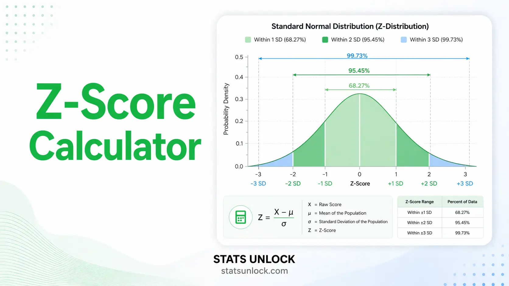
For normally distributed data: 68% of values fall within Z ±1, 95% within Z ±2, and 99.7% within Z ±3. This is called the empirical rule or the 68-95-99.7 rule.

Z-Score Calculator – Standard Score & Percentile Rank Tool

Z-Score Calculator — Standard Score & Percentile Rank Tool

📥

Data Input

Dataset (one value per line, or comma-separated)

✓ 20 valid values detected

Supports integers, decimals, negatives. Separators: comma, space, newline.

Upload CSV or Excel file:

Supports .csv, .txt, .xlsx, .xls — headers detected automatically.

Enter a single value with known mean and standard deviation to get an instant Z-score.

Value (x)

Mean (μ)

Std Dev (σ)

α significance level:

Reference

Z-Score to Percentile Table

Standard normal table — area to the left of Z (cumulative probability). Highlighted values are commonly referenced in statistics.

Guide

When to Use Z-Scores

You want to compare values from datasets with different units or scales
You need to identify outliers in a continuous variable
You want to know where a single value ranks within a distribution
You are standardizing predictors before regression or machine learning
You are working with a large sample (n ≥ 30) or known population σ
You need to compute a one-sample z-test statistic

✅ Use Z-Scores When

Data is continuous and numeric
Distribution is approximately normal
Comparing across different scales
Detecting statistical outliers

⚠️ Use Caution When

Sample size is very small (n < 10)
Distribution is heavily skewed
Data contains ordinal or categorical values
Outliers inflate the standard deviation

📊 Real-World Examples

Standardizing exam scores
Quality control in manufacturing
Clinical lab reference ranges
Financial risk z-scores (Altman Z)

🔄 Decision Tree

Need relative ranking → Z-score
Unknown σ, small n → use t-score
Skewed data → use IQR / median
Categorical data → chi-square

Tutorial

How to Use This Tool — 10 Steps

Choose your input method

Use the tabs to paste data, upload a file, or enter a single value manually.

Load a sample dataset (optional)

Use the dropdown to explore pre-loaded datasets (heights, scores, temperatures, weights, reaction times).

Paste or type your data

Enter numbers separated by commas, spaces, or newlines. Decimals and negatives are supported.

Upload a file (optional)

Upload .csv, .txt, .xlsx, or .xls files. A column picker will appear for multi-column files.

Set significance level

Choose α = 0.05, 0.01, or 0.10. This determines the outlier classification threshold.

Click "Run Z-Score Analysis"

The tool calculates Z-scores, percentiles, probability values, and outlier status for every data point.

Read the Key Statistics panel

Review mean, SD, min/max Z-score, and the count of outliers flagged in your dataset.

Explore the charts

The dot-plot shows Z-scores relative to ±1, ±2, ±3 bands; the curve shows where your data falls on the normal distribution.

Use the writing examples

Copy APA, thesis, or plain-language report text with your actual numbers pre-filled.

Export your results

Download as .txt, .xlsx, .docx, or PDF. All exports include the full Z-score table and interpretation.

Worked Example: Dataset: exam scores [55, 70, 82, 90, 65, 78, 88, 44, 95, 73]. Mean = 74, SD = 15.2. Score of 44 → Z = (44−74)/15.2 = −1.97. Percentile ≈ 2.4th. This student scored in the bottom 2.4% of the class — a mild outlier.

FAQ

Frequently Asked Questions

What is a Z-score in statistics? ›

A Z-score (also called a standard score) measures how many standard deviations a specific value lies above or below the mean of a dataset. The formula is Z = (x − μ) / σ. A Z-score of 0 means the value equals the mean; +1 means one standard deviation above; −2 means two standard deviations below.

How do you calculate a Z-score step by step? ›

Step 1: Find the mean (μ) by summing all values and dividing by n. Step 2: Calculate the standard deviation (σ) — find each value's squared deviation from the mean, average them, and take the square root. Step 3: Subtract the mean from your target value. Step 4: Divide by the standard deviation. That result is the Z-score.

What is a good Z-score? ›

In most academic and scientific contexts, Z-scores between −2 and +2 are considered "normal" (covering approximately 95.45% of normally distributed data). Whether a high or low Z-score is "good" depends on context — in exam scores a high positive Z is desirable; in clinical biomarkers, extreme values in either direction may signal abnormality.

How do I convert a Z-score to a percentile? ›

Use the standard normal cumulative distribution function (CDF), often denoted Φ(Z). The percentile = Φ(Z) × 100. For example, Z = 1.0 → Φ(1.0) = 0.8413 → 84.13th percentile. This tool calculates percentiles automatically for every value in your dataset.

What does a negative Z-score mean? ›

A negative Z-score means the raw value is below the mean. For example, Z = −1.5 means the value is 1.5 standard deviations below the mean and falls at approximately the 6.7th percentile — meaning only 6.7% of values in a normal distribution are lower.

Should I use population or sample standard deviation for Z-scores? ›

Use population SD (σ, denominator n) when you have data for the entire population. Use sample SD (s, denominator n−1, Bessel's correction) when working with a sample drawn from a larger population. This tool uses sample SD (n−1) by default, which is appropriate for most research contexts. For population data, the difference becomes negligible when n ≥ 30.

How do Z-scores help identify outliers? ›

Values with |Z| > 2 are mild outliers (falling outside 95.45% of normally distributed data), and |Z| > 3 are extreme outliers (falling outside 99.73%). This tool flags each data point as Normal, Mild Outlier, or Extreme Outlier based on its Z-score, making outlier detection instant and consistent.

What is the difference between Z-score and T-score? ›

A Z-score uses the known population standard deviation and the standard normal distribution. A T-score (not the t-statistic) is a rescaled Z: T = 50 + 10·Z, giving a mean of 50 and SD of 10 — avoiding negative values. The t-statistic (used in t-tests) is similar to Z but uses sample SD and follows a t-distribution with heavier tails, especially for small samples.

What is the 68-95-99.7 rule (Empirical Rule)? ›

For a normally distributed dataset: approximately 68.27% of values fall within Z = ±1 (one SD from the mean), 95.45% within Z = ±2, and 99.73% within Z = ±3. This rule lets you quickly estimate how unusual a value is without looking up a table — any value beyond ±3 SDs is extremely rare (less than 0.3% probability).

Can I use Z-scores with non-normal data? ›

You can compute Z-scores for any numeric dataset, but the percentile interpretations (based on the standard normal CDF) only hold when data is approximately normally distributed. For heavily skewed data, consider using median-based measures like the modified Z-score (using MAD: Z = 0.6745·(x − median)/MAD) for more robust outlier detection.

Literature

References

The Z-score calculator and its standard score interpretations are grounded in classical descriptive statistics and inferential methodology. The following references support the formulas, percentile conversions, and outlier criteria implemented in this tool.

Field, A. (2018). Discovering statistics using IBM SPSS statistics (5th ed.). SAGE Publications. https://doi.org/10.1177/0013164418776504
Tabachnick, B. G., & Fidell, L. S. (2019). Using multivariate statistics (7th ed.). Pearson. ISBN: 978-0134790541.
Zar, J. H. (2010). Biostatistical analysis (5th ed.). Prentice Hall. ISBN: 978-0131008465.
Cohen, J. (1988). Statistical power analysis for the behavioral sciences (2nd ed.). Lawrence Erlbaum Associates. https://doi.org/10.4324/9780203771587
Abdi, H. (2007). Z-scores. In N. J. Salkind (Ed.), Encyclopedia of measurement and statistics. SAGE Publications. https://doi.org/10.4135/9781412952644
Iglewicz, B., & Hoaglin, D. C. (1993). How to detect and handle outliers. ASQC Quality Press. ISBN: 978-0873892476.
Tukey, J. W. (1977). Exploratory data analysis. Addison-Wesley. ISBN: 978-0201076165.
Moore, D. S., McCabe, G. P., & Craig, B. A. (2021). Introduction to the practice of statistics (10th ed.). W. H. Freeman. ISBN: 978-1319269357.
R Core Team. (2024). R: A language and environment for statistical computing. R Foundation for Statistical Computing. https://www.R-project.org/
Altman, E. I. (1968). Financial ratios, discriminant analysis and the prediction of corporate bankruptcy. Journal of Finance, 23(4), 589–609. https://doi.org/10.1111/j.1540-6261.1968.tb00843.x
Bland, J. M., & Altman, D. G. (1996). Statistics notes: Measurement error. BMJ, 313(7059), 744. https://doi.org/10.1136/bmj.313.7059.744
Grambsch, P. M., & Therneau, T. M. (1994). Proportional hazards tests and diagnostics based on weighted residuals. Biometrika, 81(3), 515–526. https://doi.org/10.1093/biomet/81.3.515
Montgomery, D. C., & Runger, G. C. (2018). Applied statistics and probability for engineers (7th ed.). Wiley. ISBN: 978-1119400363.