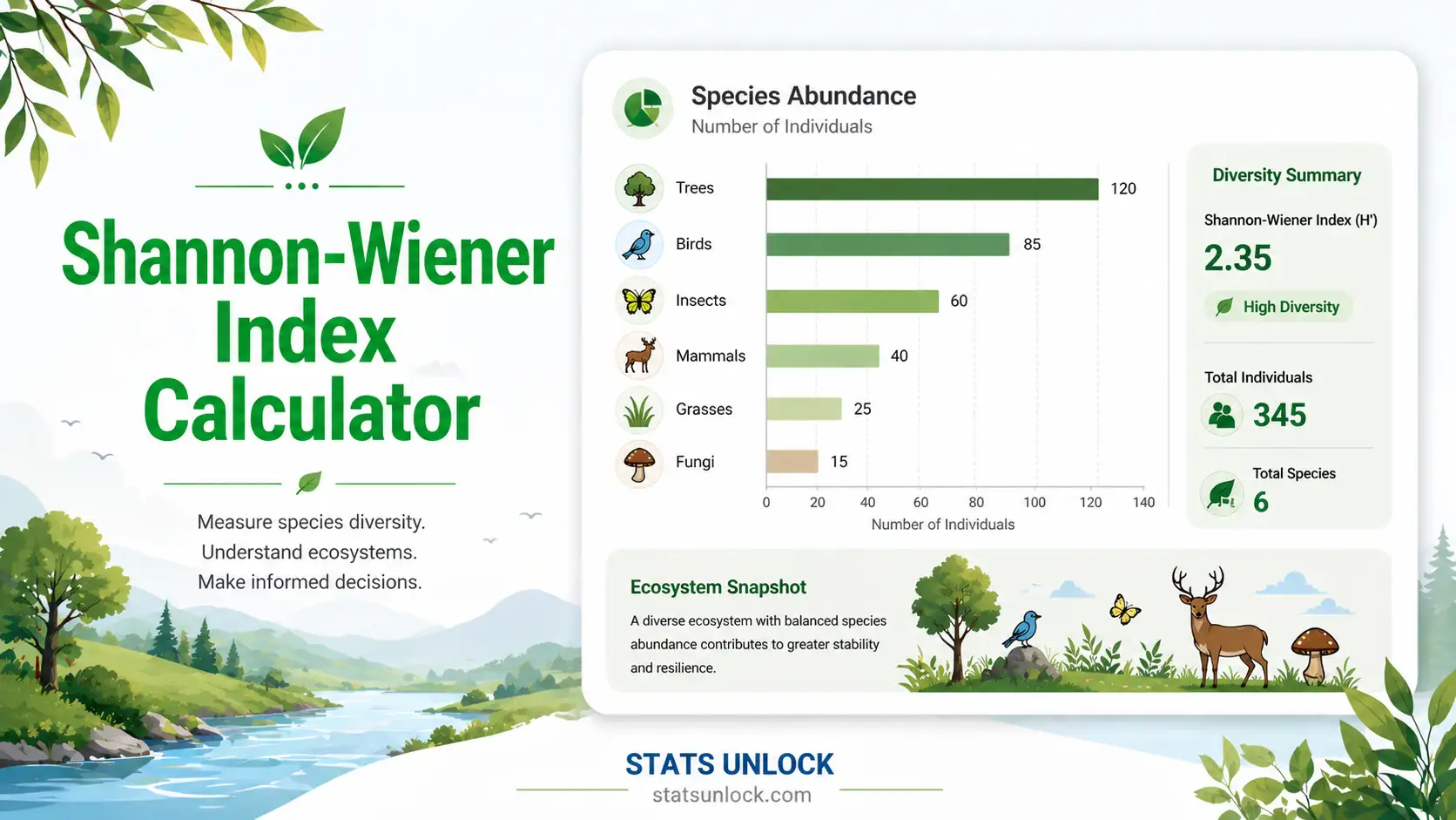
Shannon Wiener Index Calculator
A free online tool to measure species diversity (H') from your survey counts, with instant charts, evenness, richness, and publication-ready results.
🌿 Key Takeaways
- The Shannon Wiener index calculator turns your species counts into one clear diversity number (H') for ecology and wildlife studies.
- You only need the count of individuals per species. Paste them comma separated, upload a CSV file, or type them in.
- A higher H' usually means greater diversity and a healthier, more even community; a lower H' means fewer species or one dominant species.
- Typical field uses: camera trapping, point counts, vegetation plots, transects, and reef fish surveys.
- This tool also returns evenness (J'), richness (S), Simpson's index, and ready-to-paste text for reports and papers.
📥 Enter Your Data
0 values entered
🔎 Detailed Interpretation of Results
▶ Run the analysis above to generate a detailed, plain-English interpretation of your Shannon Wiener result.
✍️ How to Write Your Results in Research
▶ Run the analysis above to auto-fill all six examples with your results.
🪧 Research Poster Panel
A print-ready poster layout that updates with your result. Copy the text or use the visual scaffold for A0 / A1 conference posters.
▶ Run the analysis above to build your poster panel.
📊 Example Results
Scenario 1 — High-diversity tropical forest
A bird survey records 28 species and 412 individuals with fairly even counts. H' works out to about 3.28. This high value points to an intact, species-rich community typical of undisturbed lowland forest.
Scenario 2 — Disturbed, degraded site
A logged fragment holds just 6 species and 200 individuals, but one species makes up 150 of them. H' drops to about 0.98. The low value reflects strong dominance and reduced ecological integrity.
Scenario 3 — Same richness, different evenness
Two plots each have 5 species. Plot A counts are 20,20,20,20,20 (H' = 1.61); Plot B counts are 80,5,5,5,5 (H' = 0.76). Same richness, very different diversity — this is exactly what the Shannon Wiener index reveals.
Scenario 4 — Before vs after restoration
A grassland plot rises from H' = 1.9 before management to H' = 2.6 three years after invasive removal. The gain shows recovering evenness as native species return.
Scenario 5 — Camera-trap mammal survey
Across 1,400 trap nights, 8 mammal species are detected with counts 40,35,30,25,20,15,10,5. H' = 1.96, a moderate value for a mid-sized mammal community in a wildlife corridor.
Scenario 6 — Edge case / caution
Only 3 individuals across 3 species gives H' = 1.10, but the sample is far too small to trust. Always collect at least 30 individuals before reporting a Shannon Wiener value.
🥾 Collecting Your Species Data in the Field: A Simple Step-by-Step Guide
The Shannon Wiener index is only as good as the counts you feed it. Follow these ready-to-use steps in the field to collect clean, comparable species abundance data. Print this list and take it with you.
- Define your question first. Decide what you are comparing (site vs site, season vs season, before vs after) before you collect a single count. This sets your sampling design.
- Pick one taxonomic group and stick to it. Count only birds, only trees, or only mammals. Mixing groups makes the index meaningless.
- Choose a standard sampling method and use it everywhere: point counts, line transects, quadrats, camera traps, pitfall traps, or mist nets. Do not switch methods between sites.
- Fix your sampling effort. Keep the same transect length, plot size, count duration, or number of trap nights at every site so results are comparable.
- Set a minimum sample. Aim for at least 30 individuals and several species per sample; small samples give unstable, misleading H' values.
- Use replicates. Place at least 3 stations, plots, or transects per site so you can estimate variation and run statistics later.
- Mark station locations with GPS. Record coordinates (to a few metres) so the exact spot can be resurveyed in future years.
- Record every individual, not just species presence. The index needs abundance counts. Tally each animal or plant, not just a species checklist.
- Count during a consistent time window. Survey birds in the first hours after dawn; keep the same window and avoid rain, high wind, or extreme heat.
- Avoid double-counting. Move in one direction, note flying birds separately, and use a set detection radius so the same individual is not tallied twice.
- Log detection method. Note whether each record was seen, heard, trapped, or photographed; this matters for later corrections.
- Identify to species where possible. If you cannot, use a consistent morphospecies label (e.g. "Warbler sp. 1") and keep it identical across all sheets.
- Use a prepared datasheet. Columns: Date, Site, Station, Observer, Species, Count, Detection type, Notes. One row per species per station.
- Record effort metadata on every sheet: start and end time, weather, observer name, and equipment used. You will need these to standardise later.
- Photograph or voucher tricky species. A quick phone photo settles identification disputes back at the desk.
- Enter counts as whole numbers. The tool needs raw individual counts, not percentages or densities. Keep any conversions for a separate column.
- Back up your data the same day. Photograph paper sheets or type counts into a spreadsheet each evening so nothing is lost.
- Keep a field notebook for anything unusual: disturbance, human activity, unexpected species, or equipment problems.
- Sum counts per species before entry. Add up all stations for a site, then paste the per-species totals into this calculator (for example
52, 48, 55, 61, 47). - Never invent or round zeros away. A species truly absent from the sample is simply not listed; do not pad the data.
🧭 When to Use This Tool
- ✓ You have species count / abundance data from a defined sampling area or effort
- ✓ You want to compare diversity across sites, seasons, or treatments
- ✓ Your sampling effort is standardised (equal trap nights, transect length, area)
- ✓ You need a publication-ready diversity metric for a journal or report
- ✗ Do NOT use if effort differs greatly between sites — standardise or use rarefaction first
- ✗ Do NOT use if you only have a species list without abundances — use Species Richness
- ✗ Do NOT use with presence/absence only data — Shannon needs counts
Real-world examples: mammal diversity across a disturbance gradient using camera traps; point counts before and after reforestation; reef fish diversity across depth zones; plant diversity in grassland plots under different grazing regimes.
Sampling guidance: aim for at least 30 individuals and several species; use at least 3 replicate stations per site; apply rarefaction when comparing sites with unequal effort.
📘 How to Use This Tool — Step by Step
- Enter your data — paste counts like
52, 48, 55, 61, 47, upload a CSV file, or type them in the manual table. - Pick a sample dataset if you want to test the tool — five ecological datasets are built in.
- Configure settings — set the site name, group label, log base (ln is standard), and decimal places.
- Run the analysis — click Calculate to compute H', evenness, richness, and Simpson's index.
- Read the summary cards — green = high diversity, amber = moderate, red = low/concern.
- Read the full results table — check each value and its description.
- Examine all four charts — rank-abundance, proportional abundance, per-species contribution, and the diversity profile.
- Read the ecological interpretation — use it for park reports or journal papers.
- Copy a reporting example — six styles from journal to policy brief to poster.
- Export your results — Download Doc for a text report, or Download PDF for printing.
Worked example: a dry-season bird survey at 15 stations records 28 species and 412 individuals, returning H' = 3.28 — high diversity consistent with intact forest.
🔍 Conclusion
❓ Frequently Asked Questions
📚 References
The following references support the ecological methods used in this Shannon Wiener diversity index calculator, covering biodiversity measurement, species diversity, and best practices in ecological sampling and wildlife analysis.
- Shannon, C. E., & Weaver, W. (1949). The mathematical theory of communication. University of Illinois Press.
- Simpson, E. H. (1949). Measurement of diversity. Nature, 163, 688. doi.org/10.1038/163688a0
- Magurran, A. E. (2004). Measuring biological diversity. Blackwell Publishing.
- Krebs, C. J. (1999). Ecological methodology (2nd ed.). Benjamin Cummings.
- Hill, M. O. (1973). Diversity and evenness: A unifying notation and its consequences. Ecology, 54(2), 427–432. doi.org/10.2307/1934352
- Jost, L. (2006). Entropy and diversity. Oikos, 113(2), 363–375. doi.org/10.1111/j.2006.0030-1299.14714.x
- Pielou, E. C. (1966). The measurement of diversity in different types of biological collections. Journal of Theoretical Biology, 13, 131–144. doi.org/10.1016/0022-5193(66)90013-0
- Chao, A., & Jost, L. (2012). Coverage-based rarefaction and extrapolation. Ecology, 93(12), 2533–2547. doi.org/10.1890/11-1952.1
- Oksanen, J., et al. (2022). vegan: Community ecology package. R package v2.6-4. CRAN.R-project.org/package=vegan
- Bibby, C. J., Burgess, N. D., Hill, D. A., & Mustoe, S. H. (2000). Bird census techniques (2nd ed.). Academic Press.
- Gotelli, N. J., & Colwell, R. K. (2001). Quantifying biodiversity: Procedures and pitfalls. Ecology Letters, 4(4), 379–391. doi.org/10.1046/j.1461-0248.2001.00230.x
- Colwell, R. K. (2013). EstimateS: Statistical estimation of species richness (v9). purl.oclc.org/estimates
- Whittaker, R. H. (1972). Evolution and measurement of species diversity. Taxon, 21(2/3), 213–251. doi.org/10.2307/1218190
- R Core Team. (2024). R: A language and environment for statistical computing. R-project.org
- Ahumada, J. A., et al. (2011). Community structure and diversity of tropical forest mammals. Phil. Trans. R. Soc. B, 366(1578), 2703–2711. doi.org/10.1098/rstb.2011.0115
- Chao, A., et al. (2014). Rarefaction and extrapolation with Hill numbers. Ecological Monographs, 84(1), 45–67. doi.org/10.1890/13-0133.1
- Niedballa, J., et al. (2016). camtrapR: An R package for camera trap data. Methods Ecol. Evol., 7(12), 1457–1462. doi.org/10.1111/2041-210X.12600
- Hsieh, T. C., Ma, K. H., & Chao, A. (2016). iNEXT: rarefaction and extrapolation of Hill numbers. Methods Ecol. Evol., 7(12), 1451–1456. doi.org/10.1111/2041-210X.12613
- Roswell, M., Dushoff, J., & Winfree, R. (2021). A conceptual guide to measuring species diversity. Oikos, 130(3), 321–338. doi.org/10.1111/oik.07202
- Jost, L. (2007). Partitioning diversity into independent alpha and beta components. Ecology, 88(10), 2427–2439. doi.org/10.1890/06-1736.1