Pearson Correlation Calculator
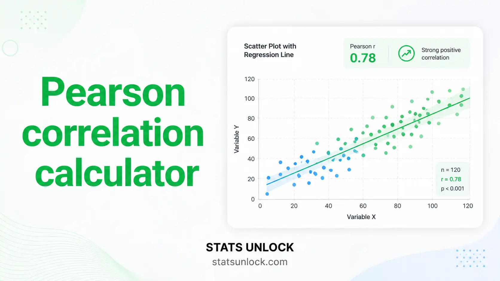
Measure the linear association between two continuous variables. Get Pearson r, r², t-statistic, p-value, Fisher's z confidence interval, scatter plot with regression line, and five APA-ready reporting templates — free, no software needed.
| Variable X | Variable Y |
|---|
Pearson Correlation Formulas
Technical Notes
- Fisher's z-transformation: Required for CI computation because r is bounded [−1, +1] and its sampling distribution is skewed, especially for |r| near 1. Fisher's z is approximately normally distributed with SE = 1/√(n−3), enabling standard CI construction.
- Significance test: The t-statistic tests H₀: ρ = 0 (no linear association in the population). For large n, even very small r values can be significant — always report r² and the CI, not just the p-value.
- r² interpretation: r² represents the proportion of variance in Y explained by X (and vice versa, since correlation is symmetric). It does not imply directionality or causation.
- Outliers: A single extreme data point can dramatically inflate or deflate r. Always inspect the scatter plot before interpreting the correlation coefficient.
- Non-linear relationships: Pearson r measures linear association only. A perfect U-shaped relationship yields r ≈ 0. Use Spearman ρ for monotonic non-linear relationships.
- Restriction of range: Sampling from a restricted range of X or Y attenuates r toward zero — the true population correlation may be larger.
Determine how many observations you need to reliably detect a correlation of a given magnitude, or check the power of your current study.
r Effect Size Reference (Cohen, 1988)
| Label | |r| | r² | Meaning | Required n (α=.05, 80% power) |
|---|---|---|---|---|
| Negligible | < 0.10 | < .01 | No meaningful linear association | > 782 |
| Small | 0.10 | .01 | Weak — barely detectable in most practical settings | 782 |
| Medium | 0.30 | .09 | Moderate — noticeable in a scatter plot | 85 |
| Large | 0.50 | .25 | Strong — clearly visible linear trend | 29 |
| Very Large | ≥ 0.70 | ≥ .49 | Very strong — near-perfect linear relationship | 13 |
Pearson r answers: "How strongly and in what direction are two continuous variables linearly associated?" It is the most widely reported measure of bivariate association in quantitative research.
Decision Checklist
- ✅Both variables are continuous (interval or ratio scale)
- ✅The relationship is expected to be linear (check scatter plot first)
- ✅Both variables are approximately normally distributed (or n ≥ 30)
- ✅No severe outliers that would distort the correlation
- ✅Observations are independent of each other
- ❌Do NOT use if the relationship is non-linear → use Spearman ρ or polynomial regression
- ❌Do NOT use if one variable is ordinal → use Spearman ρ or Kendall's τ
- ❌Do NOT use for prediction/causation → use Simple Linear Regression
- ❌Do NOT use with extreme outliers without investigation → remove, explain, or use Spearman ρ
Real-World Examples
Correlating body mass index (BMI) with systolic blood pressure across patients, to quantify how strongly weight status is linearly associated with cardiovascular risk.
Correlating the number of hours students spend studying with their final exam scores, to assess whether study time is a reliable predictor of academic performance.
Correlating mean annual temperature with glacier retreat distance across geographic regions, to quantify the linear association between climate variables.
Correlating advertising spend with monthly sales revenue to determine how strongly marketing investment is linearly related to business performance.
Related Tests — Decision Tree
What is Pearson correlation (r) and what does it measure?
Pearson's r measures the strength and direction of the linear relationship between two continuous variables. It ranges from −1 (perfect negative linear relationship) to +1 (perfect positive linear relationship). A value of 0 indicates no linear association — though a non-linear relationship may still exist. It does not establish causation.
How do I interpret the value of Pearson r?
Common benchmarks (Cohen, 1988): small = 0.10, medium = 0.30, large = 0.50. In absolute terms: |r| < 0.10 = negligible; 0.10–0.29 = weak; 0.30–0.49 = moderate; 0.50–0.69 = strong; 0.70–0.89 = very strong; ≥ 0.90 = near-perfect. The sign indicates direction: positive r = both variables tend to increase together; negative r = as one increases, the other tends to decrease. Always report r alongside r² and the confidence interval.
What is r² (coefficient of determination)?
r² is the square of Pearson r and represents the proportion of variance in Y explained by (linearly associated with) X. For example, r = 0.60 gives r² = 0.36, meaning 36% of the variance in Y is accounted for by the linear association with X. r² ranges from 0 to 1 and is always non-negative, making it a useful complement to r when communicating effect size.
What assumptions does Pearson correlation require?
(1) Both variables must be continuous. (2) The relationship should be linear — inspect the scatter plot first. (3) Both variables should be approximately normally distributed, especially for small samples. (4) No extreme outliers. (5) Independent observations. If any of these are violated, consider Spearman ρ (robust to non-normality and ordinal data) or removing/investigating outliers.
How is the p-value computed for Pearson r?
The significance of r is tested using t = r√(n−2) / √(1−r²), with df = n−2. This t-statistic follows a t-distribution under H₀: ρ = 0. The p-value is the probability of observing |r| this extreme if the true population correlation is zero. For large n, even small r can produce p < .05 — always report r² alongside p to convey practical importance.
Why use Fisher's z-transformation for the confidence interval?
Pearson r is bounded between −1 and +1, so its sampling distribution is asymmetric and skewed, especially when |r| is large. Fisher's z = atanh(r) = 0.5 × ln((1+r)/(1−r)) transforms r to an approximately normal distribution with SE = 1/√(n−3). The CI is computed on the z scale and then back-transformed to r. This gives accurate CI bounds across the full range of r.
What is the difference between Pearson and Spearman correlation?
Pearson r measures linear association and assumes bivariate normality. Spearman ρ measures monotonic association (applies Pearson r to the ranks) and makes no distributional assumption. Use Spearman when: data are ordinal, the relationship is non-linear but monotonic, or outliers are present. Pearson is more powerful when its assumptions hold; Spearman is more robust when they do not.
How do I report Pearson r in APA 7th edition format?
Format: "There was a [positive/negative] [weak/moderate/strong] correlation between X and Y, r(df) = ___, p [ Rules: italicise r and p; df = n−2 in parentheses after r; report exact p-value (p < .001 when very small); always include r², n, and 95% CI. Run the analysis above to get five auto-filled reporting templates.
Does a significant Pearson r imply causation?
No. A significant r shows that two variables are linearly associated, but does not tell you which causes which, or whether a third variable causes both. Correlation ≠ causation. Confounding variables (lurking variables), reverse causation, and spurious coincidence are all alternative explanations for any observed correlation. Only a randomised controlled experiment can support causal claims.
How many observations do I need for a reliable Pearson correlation?
Rule of thumb: n ≥ 30 for stable estimates. For 80% power to detect a medium correlation (r = 0.30) at α = 0.05 (two-tailed), approximately 85 observations are needed. For a large effect (r = 0.50), approximately 29 suffice. With n < 10, r is highly unstable and one data point can dramatically change the result. Use the power calculator on this page for exact values based on your expected r.
The following references support the statistical methods used in this calculator, covering effect size benchmarks, Fisher's z-transformation, and best practices in correlation reporting and significance testing.
- Pearson, K. (1895). Note on regression and inheritance in the case of two parents. Proceedings of the Royal Society of London, 58, 240–242. https://doi.org/10.1098/rspl.1895.0041
- Fisher, R. A. (1915). Frequency distribution of the values of the correlation coefficient in samples from an indefinitely large population. Biometrika, 10(4), 507–521. https://doi.org/10.1093/biomet/10.4.507
- Cohen, J. (1988). Statistical power analysis for the behavioral sciences (2nd ed.). Lawrence Erlbaum Associates.
- American Psychological Association. (2020). Publication manual of the American Psychological Association (7th ed.). https://doi.org/10.1037/0000165-000
- Field, A. (2018). Discovering statistics using IBM SPSS statistics (5th ed.). SAGE Publications.
- Gravetter, F. J., & Wallnau, L. B. (2021). Statistics for the behavioral sciences (10th ed.). Cengage Learning.
- Cumming, G. (2014). The new statistics: Why and how. Psychological Science, 25(1), 7–29. https://doi.org/10.1177/0956797613504966
- Lakens, D. (2013). Calculating and reporting effect sizes to facilitate cumulative science. Frontiers in Psychology, 4, 863. https://doi.org/10.3389/fpsyg.2013.00863
- Wasserstein, R. L., & Lazar, N. A. (2016). The ASA statement on p-values. The American Statistician, 70(2), 129–133. https://doi.org/10.1080/00031305.2016.1154108
- Hauke, J., & Kossowski, T. (2011). Comparison of values of Pearson's and Spearman's correlation coefficients on the same sets of data. Quaestiones Geographicae, 30(2), 87–93. https://doi.org/10.2478/v10117-011-0021-1
- R Core Team. (2024). R: A language and environment for statistical computing. https://www.R-project.org/
- Virtanen, P., et al. (2020). SciPy 1.0. Nature Methods, 17, 261–272. https://doi.org/10.1038/s41592-019-0686-2
- NIST/SEMATECH. (2013). e-Handbook of statistical methods. https://www.itl.nist.gov/div898/handbook/


