Mean (Average) Calculator Report
Generated by STATS UNLOCK — statsunlock.com
1. Analysis Overview
2. Data Summary
3. Statistical Results
4. Interpretation
5. APA Reporting
6. Assumption Checks
7. References
See the online Mean Calculator at statsunlock.com for full references.
Mean Calculator — Free Online Average Calculator
Compute arithmetic mean, median, mode, standard deviation, SEM, CV, skewness & more — instantly, with step-by-step results and charts.
This mean calculator (also called an arithmetic mean calculator) helps students, researchers, analysts, and educators quickly calculate the average of any dataset. Enter your numbers, adjust settings, and get instant results including mean, median, mode, standard deviation, variance, SEM, and coefficient of variation — all with a clear step-by-step explanation. Export to Word, PDF, or Excel in one click.
| Statistic | Value | Description |
|---|
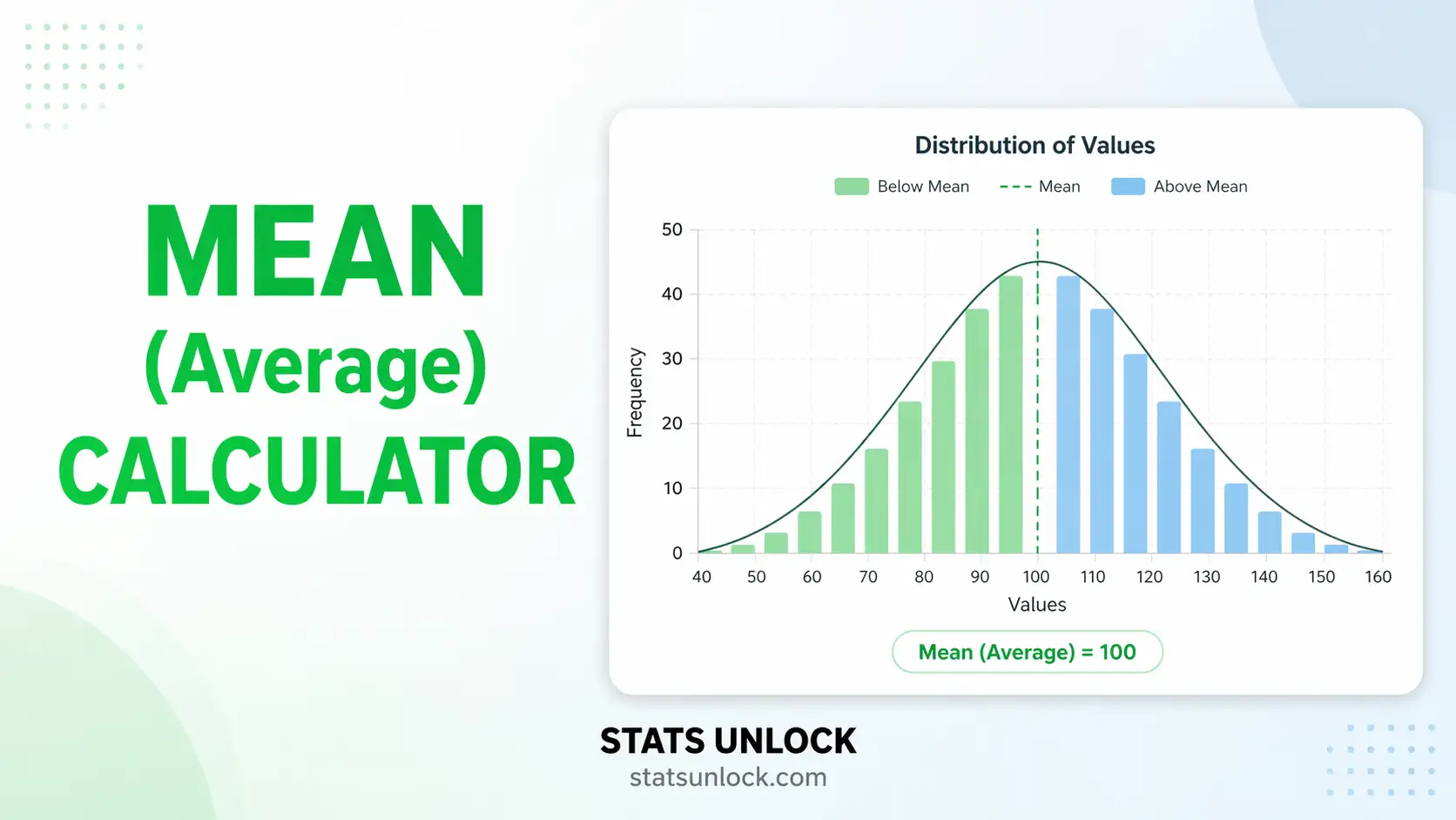
Distribution — Histogram & KDE
Box Plot — Spread & Outliers
A. Formulas Used
B. Technical Notes
- Bessel's Correction — sample variance divides by (n−1) to give an unbiased estimator of population variance.
- Sensitivity to outliers — the arithmetic mean is not robust; a single extreme value can shift it substantially. Compare mean vs trimmed mean and median to assess outlier influence.
- Central Limit Theorem — for n ≥ 30, the sampling distribution of x̄ approaches normality regardless of the population distribution.
- Skewness interpretation — |g₁| < 0.5 = approximately symmetric; 0.5–1.0 = moderate skew; > 1.0 = substantial skew.
- Kurtosis — excess kurtosis > 0 indicates heavier tails than normal (leptokurtic); < 0 indicates lighter tails (platykurtic).
The arithmetic mean is appropriate when you have continuous or discrete numerical data that is reasonably symmetric and free of severe outliers. It is the most common measure of central tendency in statistics, science, education, and business.
- Your data is numerical (interval or ratio scale)
- Distribution is approximately symmetric
- No extreme outliers distorting the average
- You need a single representative value for the dataset
- You are estimating a population mean from a sample
- Data is categorical or nominal → use Mode instead
- Distribution is heavily skewed → consider Median
- Data contains rates or ratios → consider Geometric Mean
📚 Education
Average exam scores for a class of students to track academic performance.
🌡️ Science
Mean daily temperature over a month for climate or environmental analysis.
💰 Business
Average monthly sales across branches to benchmark regional performance.
🏥 Medicine
Mean blood pressure readings from a patient cohort in a clinical trial.
Q1. What is the mean in statistics?
The mean (or arithmetic mean) is the sum of all values in a dataset divided by the number of values. It is the most widely used measure of central tendency. For example, the mean of [4, 6, 8, 10] = 28 / 4 = 7. It tells you the "average" or "typical" value of a dataset.
Q2. How do I calculate the mean step by step?
Step 1: Add all values together (Σxᵢ). Step 2: Count the number of values (n). Step 3: Divide the sum by the count: x̄ = Σxᵢ / n. Example: [10, 20, 30] → Sum = 60, n = 3, Mean = 60/3 = 20. This calculator shows every step automatically.
Q3. What is the difference between mean, median, and mode?
The mean is the arithmetic average (sum / count). The median is the middle value when data is sorted — it is resistant to outliers. The mode is the most frequently occurring value. For symmetric data, all three are similar. For skewed data, they diverge significantly.
Q4. How does an outlier affect the mean?
Outliers pull the mean toward them. For example, if nine students scored 60–80 on a test but one scored 0, the mean drops significantly. The median is unaffected. This is why comparing the mean, trimmed mean, and median is important for detecting outlier influence.
Q5. What is the difference between sample mean and population mean?
The population mean (μ) is calculated from every member of a group. The sample mean (x̄) is calculated from a subset. In practice, you almost always work with the sample mean and use it to estimate μ. The standard error of the mean (SEM) quantifies the uncertainty in this estimate.
Q6. What is the standard error of the mean (SEM)?
SEM = s / √n, where s is the sample standard deviation and n is the sample size. SEM tells you how much the sample mean would vary if you repeated the study many times. Larger samples have smaller SEM, giving more precise estimates of the population mean.
Q7. What is a 95% confidence interval for the mean?
A 95% CI means that if you repeated the study 100 times, about 95 of those intervals would contain the true population mean. It is calculated as: CI = x̄ ± t*(α/2, n−1) × SEM, where t* is the critical t-value. A narrower CI indicates higher precision.
Q8. When should I use the trimmed mean instead of the arithmetic mean?
Use the trimmed mean when your data has extreme outliers or a heavily skewed distribution. The trimmed mean removes a fixed percentage of the lowest and highest values (e.g., 5% from each end) before computing the average. This makes it resistant to outliers while remaining more sensitive than the median.
Q9. What does coefficient of variation (CV) tell me?
CV = (SD / Mean) × 100%. It expresses variability as a percentage of the mean, allowing comparison between datasets with different units. CV < 15% = low variability; 15–30% = moderate; >30% = high. It is useful in ecology, finance, and quality control.
Q10. Can this mean calculator handle large datasets?
Yes. You can type, paste, or upload a CSV file with hundreds or thousands of values. The calculator computes all statistics instantly in your browser — no data is sent to any server. For very large datasets, uploading a CSV file is the fastest input method.
- Choose a Sample Dataset (optional) Select one of the 5 built-in datasets from the dropdown to see how the calculator works before entering your own data. Example: Select "Student Exam Scores" to load 15 pre-filled scores.
- Enter Your Data Type or paste comma/space/newline-separated numbers into the text box. All three input tabs work. Example: 72, 85, 90, 68, 78, 95, 88, 74, 82, 91
- Upload a CSV (optional) Switch to the Upload tab and select a .csv file. The first column of numbers is used automatically. Headers are skipped. Example: A spreadsheet column of exam scores exported as CSV.
- Set Decimal Places Choose 2 (default) for most purposes, 3–4 for scientific data. Example: Mean = 82.30 (2 dp) vs 82.300 (3 dp).
- Choose Confidence Level Default is 95% (standard in most research). Use 99% for medical or safety-critical contexts. Example: 95% CI for mean = [79.1, 85.5].
- Set Trim Percentage Default is 5% each side. Increase to 10–20% if your data has many extreme outliers. Set to 0 to disable trimming. Example: 5% trim removes 1 value each side from a dataset of 20.
- Click "Calculate Mean & Statistics" Results appear immediately below — summary cards, full table, and visualizations. Example: Mean = 82.3, Median = 83, SD = 8.4, SEM = 2.66.
- Read the Summary Cards The top row shows the six most important statistics at a glance. Hover over the charts for interactive tooltips. Example: The histogram shows if data is bell-shaped or skewed.
- Check Assumptions The assumption panel shows whether your data meets the conditions for using the arithmetic mean reliably. Example: Green = condition met; Yellow = borderline; Blue = informational.
- Export Your Results Use the four download buttons: Word for reports, PDF for printing, Excel for further analysis, Doc for plain text. Example: Download Word to include a formatted report in your thesis.
The following references support the statistical methods used in this mean calculator tool, covering descriptive statistics, confidence interval estimation, and best practices in data analysis and reporting.
- Gauss, C. F. (1809). Theoria motus corporum coelestium. Perthes and Besser. [Origin of least-squares estimation and the arithmetic mean.]
- Fisher, R. A. (1925). Statistical methods for research workers. Oliver and Boyd.
- Cohen, J. (1988). Statistical power analysis for the behavioral sciences (2nd ed.). Lawrence Erlbaum Associates.
- Field, A. (2018). Discovering statistics using IBM SPSS statistics (5th ed.). SAGE Publications.
- Gravetter, F. J., & Wallnau, L. B. (2017). Statistics for the behavioral sciences (10th ed.). Cengage Learning.
- Moore, D. S., McCabe, G. P., & Craig, B. A. (2016). Introduction to the practice of statistics (8th ed.). W. H. Freeman.
- Cumming, G. (2014). The new statistics: Why and how. Psychological Science, 25(1), 7–29. https://doi.org/10.1177/0956797613504966
- Wilcox, R. R. (2012). Introduction to robust estimation and hypothesis testing (3rd ed.). Academic Press.
- Tukey, J. W. (1977). Exploratory data analysis. Addison-Wesley.
- American Psychological Association. (2020). Publication manual of the American Psychological Association (7th ed.). APA. https://doi.org/10.1037/0000165-000
- NIST/SEMATECH. (2013). e-Handbook of statistical methods. National Institute of Standards and Technology. https://www.itl.nist.gov/div898/handbook/
- R Core Team. (2024). R: A language and environment for statistical computing. R Foundation for Statistical Computing. https://www.R-project.org/


