What is the CV formula in statistics?

The CV formula is: CV (%) = (Standard Deviation / Mean) × 100. For a population, use population SD (σ); for a sample, use sample SD (s calculated with n−1 denominator).

How do you interpret CV results in research?

In research, CV 30% = high variability. Field-specific benchmarks vary — ecology may tolerate higher CVs than laboratory assays.

Coefficient of Variation (CV) — Descriptive Statistics Tool

Coefficient of Variation Calculator — Free CV Statistics Tool

Coefficient of Variation (CV) — Analysis Report

Generated by STATS UNLOCK — statsunlock.com

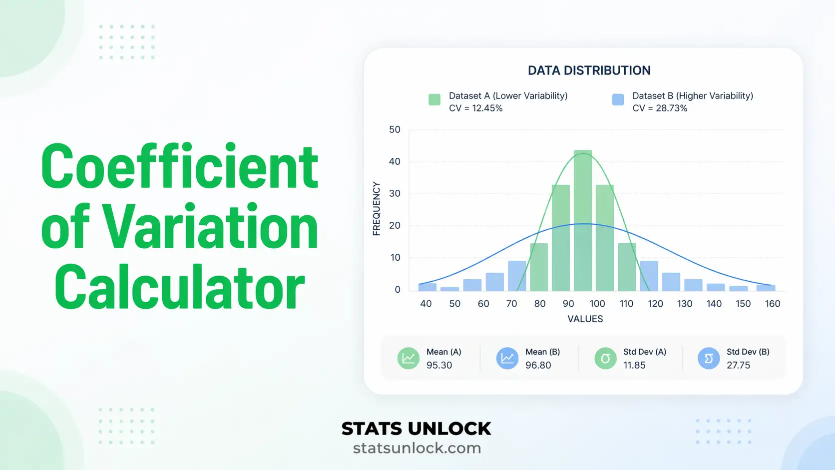
Coefficient of Variation Calculator

Free online CV statistics tool — compute CV%, SD, mean, and get full interpretation with charts and export options.

Descriptive Statistics Variability Measure Unit-Free Relative Dispersion Comparative Analysis

Data Input

Enter Data Values

Enter values to begin. Separate by commas, spaces, or new lines.

SD Type:

Upload CSV or Excel File

Supports .csv, .txt, .xlsx, .xls — headers detected automatically.

Enter Mean and Standard Deviation Directly

Mean (x̄)

SD (s)

Sample Size (n)

Use this tab if you already know the mean and SD from published data.

Results — CV Analysis

Statistic	Value	Description

Visualisations

Distribution & CV Range

Box Plot Summary

Interpretation — Results

How to Write Your Results

🔬 Technical Notes — Formulas & Definitions

CV Formula

CV (%) = (s / x̄) × 100

Where:
s = sample standard deviation (or σ for population)
x̄ = arithmetic mean
n = number of observations

Standard Deviation (Sample)

s = √[ Σ(xᵢ − x̄)² / (n−1) ]

Bessel's correction (n−1) is used to produce an unbiased
estimate of the population SD from a sample.

Relative Standard Deviation

RSD = CV (%) — These terms are interchangeable.
Both express SD as a percentage of the mean.

Confidence Interval for CV (McKay's approximation)

95% CI for CV ≈ CV × [1 ± z₀.₀₂₅ / √(2n)]

Note: This is an approximation. Exact CIs require the
non-central chi-square distribution.

Assumption Checks

✓ Positive MeanCV is only meaningful when the mean is positive and non-zero. Negative or near-zero means produce uninformative or undefined CV values.

✓ Ratio-Scale DataCV requires ratio-scale data (a true zero). It should not be used with interval-scale data (e.g., Celsius temperature, IQ scores) where zero is arbitrary.

✓ Approximately NormalCV is most interpretable for unimodal, approximately symmetric distributions. Heavily skewed data may yield misleading CV values.

✓ No Extreme OutliersOutliers inflate both the SD and, if extreme, may distort the mean, leading to artificially high CV. Check data for outliers before interpreting CV.

When to Use the Coefficient of Variation

Comparing variability between two datasets measured in different units (e.g., kg vs. cm)
Comparing variability between datasets with very different means
Evaluating assay precision or laboratory measurement consistency
Assessing ecological variability across species abundance or habitat metrics
Benchmarking financial return consistency across investment portfolios
Quality control in manufacturing — monitoring production variability

🧬 Biology / Medicine

CV <10% = high precision for assays. Used to validate lab methods and compare inter-lab reproducibility.

🌿 Ecology

Compare variability in species counts, biomass, or environmental variables across different sites or scales.

💰 Finance

Risk-adjusted return comparisons. A lower CV means more consistent returns relative to the average.

🎓 Education

Compare score variability across tests with different maximum marks or point scales.

📌 Decision Tree — Should I Use CV? Is your data measured on a ratio scale (true zero)? ──────── NO → Do NOT use CV │ YES ▼ Is your mean positive and non-zero? ────────────────────────── NO → Do NOT use CV │ YES ▼ Are you comparing datasets with different units or scales? ─── YES → ✅ Use CV │ NO ▼ Are you comparing datasets with very different means? ────────YES → ✅ Use CV │ NO ▼ Is absolute spread (same units) all you need? ───────────── YES → Use SD or IQR instead

How to Use This Tool

Choose input method — Paste/type values, upload a CSV or Excel file, or enter mean + SD directly using the Manual Entry tab.
Select or load a sample dataset — Five pre-loaded datasets cover biology, ecology, health, and social science contexts. Dataset 1 loads automatically on page render.
Choose SD type — Select Sample SD (n−1) for research data (default), or Population SD (n) if your data is the entire population.
Click Calculate — The tool instantly computes CV%, mean, SD, SEM, 95% CI for the mean, and 95% CI for the CV.
Read the Results Table — All statistics are shown with plain-language descriptions. The CV badge colour-codes low/moderate/high variability.
Interpret the charts — The distribution plot shows data spread relative to the mean. The box plot shows median, quartiles, and outliers.
Read the Interpretation section — Auto-generated paragraphs explain your specific CV value in plain language, including practical significance and limitations.
Copy a write-up — Five writing style cards (APA, thesis, plain language, abstract, pre-registration) auto-fill with your computed values. Click 📋 Copy to use them.
Check assumptions — The Assumption Checks section flags any potential issues with your data (e.g., outliers, near-zero mean).
Download your report — Export as .txt, .xlsx, .docx, or print as PDF using the four download buttons in the Results section.

Worked Example: A clinical researcher measures fasting glucose in 20 patients: mean = 98.4 mg/dL, SD = 11.7 mg/dL. CV = (11.7 / 98.4) × 100 = 11.89%. This indicates moderate variability, acceptable for clinical population studies but potentially high for a laboratory assay.

Frequently Asked Questions

What is the coefficient of variation (CV)?

The coefficient of variation (CV) is a standardised, unit-free measure of relative dispersion, calculated as CV (%) = (SD / Mean) × 100. It expresses how large the standard deviation is as a percentage of the mean, making it ideal for comparing variability across datasets with different units or scales.

How do you calculate the coefficient of variation?

To calculate CV: (1) Find the mean (x̄) of your data. (2) Calculate the standard deviation (SD or s). (3) Divide SD by the mean. (4) Multiply by 100. Formula: CV (%) = (s / x̄) × 100. This tool performs all steps automatically with a sample SD (n−1) by default.

What is a good coefficient of variation percentage?

Benchmarks depend on your field. In general: CV < 15% = low variability (precise); CV 15–30% = moderate; CV > 30% = high variability. In laboratory settings, CV < 5% is excellent, < 10% acceptable. In ecology and field biology, CV > 30% is common and acceptable.

What does a high coefficient of variation mean?

A high CV indicates that the data are widely dispersed relative to the mean. This can reflect genuine biological or ecological variability, measurement imprecision, heterogeneous populations, or outliers. Always investigate the source of high CV before drawing conclusions.

What is the difference between CV and standard deviation?

SD is an absolute measure of spread expressed in the same units as your data (e.g., kg, mg/dL). CV is a relative, unit-free percentage, making it comparable across different datasets. Use SD when absolute spread matters; use CV when you need to compare variability proportionally.

Can the coefficient of variation be negative?

CV is typically reported as an absolute (positive) value. If the mean is negative (e.g., Celsius temperatures, financial losses), the CV formula can produce a negative number. In practice, take the absolute value of both SD and mean, or avoid CV for data with negative or near-zero means.

When should I use CV instead of standard deviation?

Use CV when: (1) comparing variability between datasets measured in different units, (2) datasets have very different means making SD comparisons unfair, (3) you need a unit-free, scale-independent measure of dispersion. Use SD when you need to understand absolute spread in the original measurement units.

Is CV the same as relative standard deviation (RSD)?

Yes. Coefficient of variation (CV) and relative standard deviation (RSD) are identical statistics. Both = (SD / Mean) × 100. The term RSD is more common in analytical chemistry and laboratory science; CV is more common in statistics, biology, and social sciences.

How do you interpret CV results in ecology or wildlife research?

In ecology, CV is used to compare variability in species abundance, biomass, population density, or environmental variables across sites. A CV < 20% suggests relatively homogeneous sites; CV 20–50% indicates moderate spatial or temporal heterogeneity; CV > 50% signals high variability, which is common for rare or aggregated species.

Can I use CV to compare two datasets directly?

Yes — this is CV's primary use. Calculate CV separately for each dataset and compare. The dataset with the lower CV has less relative variability. For example, if Dataset A has CV = 12% and Dataset B has CV = 28%, Dataset A is more consistent relative to its mean, regardless of the raw units or scale.

References

The coefficient of variation calculator and its interpretation guidelines are grounded in established descriptive statistics and relative dispersion methodology. The following references support the formulas, benchmarks, and reporting standards used in this tool.

Everitt, B. S., & Skrondal, A. (2010). The Cambridge Dictionary of Statistics (4th ed.). Cambridge University Press. https://doi.org/10.1017/CBO9780511779633
Field, A. (2018). Discovering Statistics Using IBM SPSS Statistics (5th ed.). SAGE Publications.
McKay, A. T. (1932). Distribution of the coefficient of variation and the extended "t" distribution. Journal of the Royal Statistical Society, 95(4), 695–698. https://doi.org/10.2307/2342041
Reed, G. F., Lynn, F., & Meade, B. D. (2002). Use of coefficient of variation in assessing variability of quantitative assays. Clinical and Diagnostic Laboratory Immunology, 9(6), 1235–1239. https://doi.org/10.1128/cdli.9.6.1235-1239.2002
Abdi, H. (2010). Coefficient of variation. In N. J. Salkind (Ed.), Encyclopedia of Research Design. SAGE Publications. https://doi.org/10.4135/9781412961288.n51
American Psychological Association. (2020). Publication Manual of the American Psychological Association (7th ed.). https://doi.org/10.1037/0000165-000
Sokal, R. R., & Rohlf, F. J. (2012). Biometry: The Principles and Practice of Statistics in Biological Research (4th ed.). W. H. Freeman.
Bland, M. (2015). An Introduction to Medical Statistics (4th ed.). Oxford University Press.
Zar, J. H. (2010). Biostatistical Analysis (5th ed.). Pearson Prentice Hall.
Currell, G., & Dowman, A. (2009). Essential Mathematics and Statistics for Science (2nd ed.). Wiley-Blackwell.
National Institute of Standards and Technology. (2023). NIST/SEMATECH e-Handbook of Statistical Methods. https://www.itl.nist.gov/div898/handbook/
Limpert, E., Stahel, W. A., & Abbt, M. (2001). Log-normal distributions across the sciences: Keys and clues. BioScience, 51(5), 341–352. https://doi.org/10.1641/0006-3568(2001)051[0341:LNDATS]2.0.CO;2
Hendricks, W. A., & Robey, K. W. (1936). The sampling distribution of the coefficient of variation. The Annals of Mathematical Statistics, 7(3), 129–132. https://doi.org/10.1214/aoms/1177732503