Kolmogorov-Smirnov Test Calculator – Free Online K-S Test for Normality & Two-Sample Distributions

Non-Parametric · Goodness of Fit

Kolmogorov-Smirnov Test Calculator

A free online K-S test calculator for one-sample normality testing and two-sample distribution comparison. Get the D-statistic, exact p-value, ECDF visualizations, APA-formatted results, and a publication-ready report — all in one click.

D-statistic P-value ECDF Plot APA Format One-Sample Two-Sample Free Online

📥 Enter Your Data

Sample Dataset:

SAMPLE 1 n = 0

Comma-separated (default). Newline or tab also accepted.

SAMPLE 2 n = 0

Used only when Test Type = Two-Sample K-S.

📋 Expected file format Each numeric column = one sample. Always select 2 columns (Sample 1 and Sample 2). For a one-sample K-S test only Sample 1 is used; for a two-sample K-S test both are compared. Mixed/text columns are auto-skipped. Toggle "First row is a header" if your file has no header.

Upload CSV or Excel file:

Supports .csv, .txt, .xlsx, .xls. Files stay on your device — nothing is uploaded to any server.

Enter values in the editable cells below. Add or remove rows as needed.

⚙️ Test Configuration

Test Type

Alpha (α)

Alternative

Lilliefors Correction

📊 Results Summary

📈 Visualizations

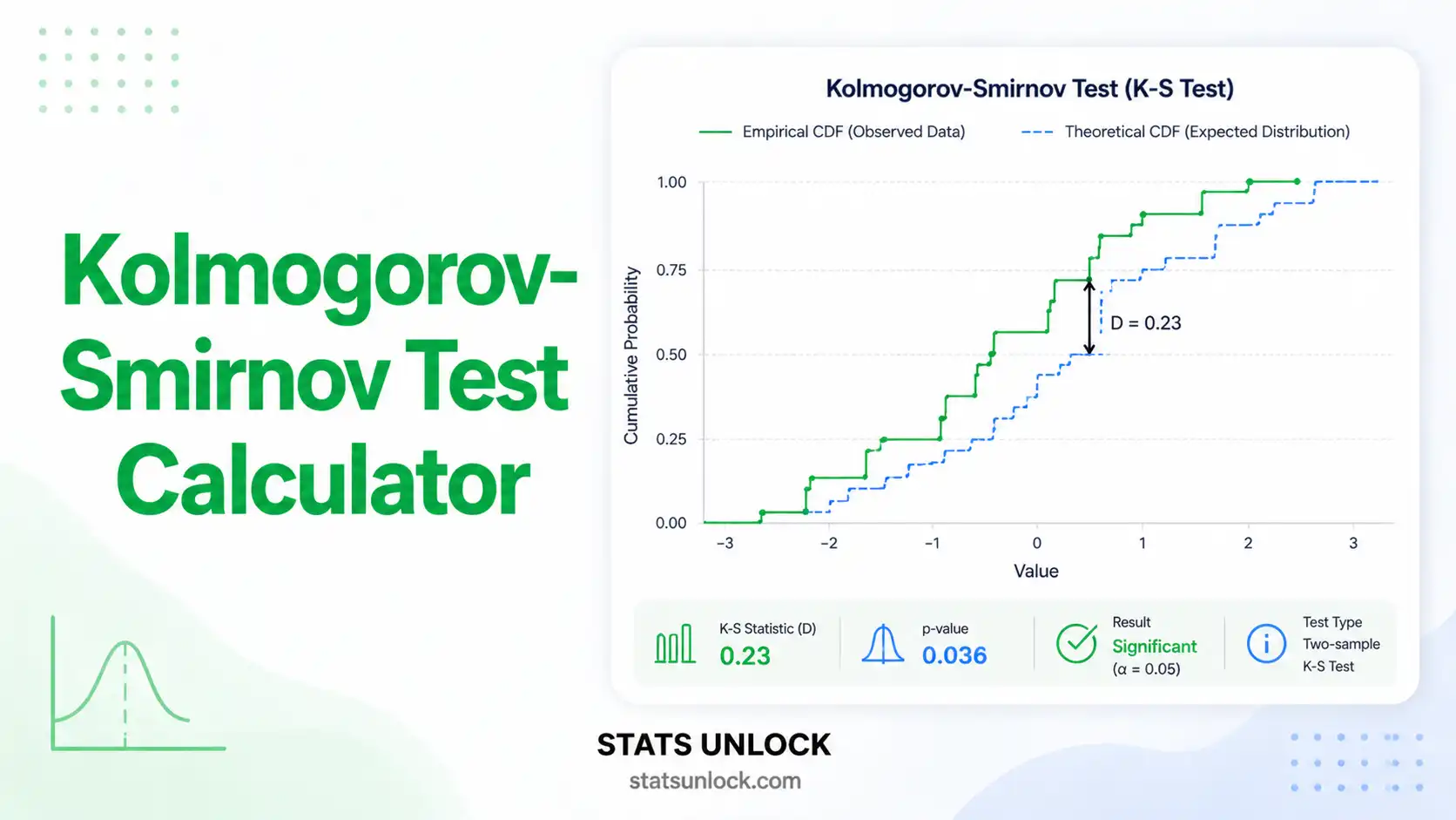
ECDF Comparison Plot

Density Curves (KDE)

🛡️ Assumption Checks

💡 Interpretation Results

📝 How to Write Your Results in Research

Five ready-to-use templates auto-filled with your computed K-S test statistics. Click 📋 Copy on any card.

🎯 Conclusion

📐 Formulas & Technical Notes

One-Sample K-S Test Statistic

D = supx | Fn(x) − F(x) |

Where:
  D       = Kolmogorov-Smirnov test statistic (supremum of vertical deviation)
  Fn(x)   = Empirical Cumulative Distribution Function (ECDF) of the sample
  F(x)    = Reference Cumulative Distribution Function (e.g., Normal(μ, σ))
  sup     = supremum (maximum over all x in the support)
  n       = sample size

Two-Sample K-S Test Statistic

Dn,m = supx | F1,n(x) − F2,m(x) |

Where:
  F1,n(x) = ECDF of Sample 1 (size n)
  F2,m(x) = ECDF of Sample 2 (size m)

Asymptotic P-value (Kolmogorov Distribution)

P( √n · D > d ) ≈ 2 · Σk=1..∞ (−1)k−1 · exp(−2 k² d²)

Effective sample size for two-sample:
  neff = (n · m) / (n + m)

Critical value approximation (α = 0.05):
  Dcrit ≈ 1.36 / √neff

Effect Size (Cliff-style for D)

D itself is bounded in [0, 1] and serves as a non-parametric effect size:
  D < 0.10  → trivial / negligible
  0.10 ≤ D < 0.20 → small
  0.20 ≤ D < 0.30 → medium
  D ≥ 0.30        → large

Technical Notes

Continuous distributions only. The classical K-S test assumes continuous reference distributions. With ties present, p-values become conservative (anti-conservative bias removed).
Lilliefors correction. When μ and σ are estimated from the same data, the standard p-value is too conservative. This calculator applies a Lilliefors-style adjustment for normality testing.
Less powerful than Shapiro-Wilk. For pure normality testing on n < 50, prefer Shapiro-Wilk. K-S is preferred for non-normal reference distributions or two-sample comparison.
Direction of K-S sensitivity. K-S is most sensitive to differences near the distribution's center and less sensitive in the tails — use Anderson-Darling for tail-sensitive tests.

🎯 When to Use This K-S Test

This free Kolmogorov-Smirnov test calculator is designed for researchers, students, and analysts who need to test whether a sample comes from a specified distribution (one-sample) or whether two independent samples come from the same distribution (two-sample).

Decision Checklist

You have one continuous variable and want to test if it follows a known distribution (Normal, Exponential, Uniform).
You have two independent samples and want to test if they come from the same distribution.
Your data are continuous (ratio or interval); ties are minimal.
Observations within each sample are independent.
Do NOT use for paired/matched data → use Wilcoxon Signed-Rank instead.
Do NOT use for purely categorical data → use Chi-Square test instead.
Do NOT prefer K-S over Shapiro-Wilk for normality testing with n < 50.

Real-World Examples

Medical Research: Test whether patient recovery times follow a normal distribution before applying a parametric ANOVA.
Education: Compare the distribution of exam scores between an in-person and an online cohort to see if grading is equivalent.
Quality Control: Verify whether daily defect counts in a manufacturing line follow a Poisson distribution.
Ecology: Compare the size distribution of a fish species between two lakes to detect habitat-driven divergence.
Finance: Test whether daily stock returns are normally distributed (a common assumption in option pricing models).

Sample Size Guidance

Minimum: n = 4 (technically valid but very low power).
Recommended: n ≥ 25 for one-sample normality; n₁ + n₂ ≥ 40 for two-sample.
For detecting medium D ≈ 0.20 at α = 0.05 with 80% power: ≈ 50 per group.

Decision Tree

Want to test distribution shape?
├─ One sample vs theoretical distribution
│  ├─ Reference is Normal, n < 50  → Shapiro-Wilk (more powerful)
│  └─ Reference is Normal, n ≥ 50  → K-S (this tool)
│  └─ Reference is non-Normal      → K-S (this tool)
└─ Two independent samples
   ├─ Compare distributions       → Two-Sample K-S (this tool)
   └─ Compare medians only        → Mann-Whitney U
   └─ Compare means (if normal)   → Independent t-test

📘 How to Use This Kolmogorov-Smirnov Test Calculator

Step 1 — Enter Your Data

Use the Paste / Type tab for quick entry (default is comma-separated, e.g., 52, 48, 55, 61, 47). For larger datasets, switch to the Upload CSV / Excel tab. The Manual Entry tab gives you a small editable spreadsheet.

Step 2 — Choose a Sample Dataset

The dropdown ships with five pre-built examples (Reaction Time, Patient Recovery, Exam Scores, Daily Sales, Plant Heights). Pick one to see the tool in action immediately.

Step 3 — Configure the Test

Pick One-Sample (compare to Normal) or Two-Sample (compare two samples). Set α (default 0.05). Use Two-sided for general "are these distributions different?" questions.

Step 4 — Click "Run K-S Test"

The tool computes the empirical CDF, calculates the D-statistic, and returns the p-value with full diagnostics in under a second.

Step 5 — Read the Summary Cards

Four colored cards display: D-statistic, p-value, sample size, and significance verdict (green = significant, red = not significant).

Step 6 — Read the Full Results Table

Statistic | Value | Description rows include D, p, n, the critical D, and the effect-size interpretation.

Step 7 — Examine the Two Charts

Chart 1: ECDF curves with the D point clearly marked. Chart 2: histogram with the reference distribution overlay so you can see where the data deviate.

Step 8 — Check the Assumptions

Open the Assumption Check panel — the tool flags ties, sample-size warnings, and tells you when Lilliefors correction is being applied.

Step 9 — Read the Interpretation

Plain-language paragraphs explain what your D and p-value mean in real terms. Pick one of the five Writing Templates to drop into your paper.

Step 10 — Export Your Report

Hit Download Doc for a plain-text report or Download PDF for a print-ready A4 document with all 8 sections.

❓ Frequently Asked Questions

Q1. What is the Kolmogorov-Smirnov test and when should I use it?

The Kolmogorov-Smirnov (K-S) test is a non-parametric test that compares an empirical distribution function to a reference distribution (one-sample) or two empirical distributions to each other (two-sample). Use it to check whether a sample is drawn from a normal distribution, or whether two samples come from the same underlying distribution. It is the most popular general-purpose distribution-comparison test in the non-parametric toolkit.

Q2. What is a p-value in the K-S test and how do I interpret it?

The p-value is the probability of observing a D-statistic at least as large as the one computed if the null hypothesis were true. A small p-value (< 0.05) means the empirical and reference distributions differ more than would be expected by chance alone. Example: p = 0.03 means there is a 3% probability of seeing this much deviation purely by chance under the null.

Q3. What is the difference between one-sample and two-sample K-S tests?

The one-sample K-S test compares one dataset to a theoretical distribution (usually Normal). The two-sample K-S test compares two datasets to each other without assuming a reference distribution. Both use the maximum vertical distance D between empirical CDFs as the test statistic. One-sample answers: "Does my data follow distribution X?" Two-sample answers: "Are these two samples from the same population?"

Q4. What does the D-statistic mean in the K-S test?

D is the supremum (maximum) of the absolute differences between the two cumulative distribution functions being compared. D ranges from 0 to 1; values close to 0 mean the distributions match closely, while values close to 1 indicate strong divergence. Cohen-style benchmarks: D < 0.10 trivial, 0.10–0.20 small, 0.20–0.30 medium, ≥ 0.30 large.

Q5. What assumptions does the Kolmogorov-Smirnov test require?

Observations must be independent and identically distributed (iid). The reference distribution must be continuous and fully specified — parameters should not be estimated from the same data unless you apply the Lilliefors correction (this tool does it automatically). With many tied values, p-values become conservative; consider an exact-permutation alternative for small samples with heavy ties.

Q6. How large a sample do I need for the K-S test?

The K-S test technically works for any n ≥ 4, but power is very low for small samples. For reliable normality detection use n ≥ 25. For two-sample tests, both n₁ and n₂ should be at least 20 for reasonable sensitivity to medium effect sizes (D ≈ 0.20). For 80% power to detect a medium effect at α = 0.05, plan for ≈ 50 observations per group.

Q7. K-S test vs Shapiro-Wilk test — which is better for normality?

Shapiro-Wilk is more powerful than K-S for detecting departures from normality, especially with n < 50. Use Shapiro-Wilk as the default normality test when n ≤ 50. Use K-S when (a) you need to compare against a non-normal reference distribution, (b) you have a very large sample, or (c) you need to compare two empirical samples directly.

Q8. What is the Lilliefors correction in K-S testing?

When you estimate the mean and SD from your data and then run a one-sample K-S test for normality, the standard p-values are too conservative (you would fail to reject normality too often). Lilliefors (1967) provided corrected critical values that account for this estimation. This calculator applies the Lilliefors approximation automatically in "Auto" mode whenever you run a one-sample test against Normal with parameters estimated from the data.

Q9. How do I report Kolmogorov-Smirnov test results in APA format?

APA 7th edition format: D(n) = value, p = value. Example: "A one-sample Kolmogorov-Smirnov test indicated that the data did not deviate significantly from a normal distribution, D(50) = .082, p = .421." Always report sample size, exact D, and exact p-value (use "p < .001" for very small values; never write "p = 0.000"). See the auto-filled APA template in the How to Write Your Results section above.

Q10. What if my K-S test result is non-significant — does it prove normality?

No. A non-significant K-S result (p > 0.05) only means there is insufficient evidence to reject normality — it does not prove the data are normal. This is especially true for small samples where power is low. Combine the K-S test with a Q-Q plot, histogram, and Shapiro-Wilk test for a complete normality assessment. If you need to quantify evidence in favor of normality, consider a Bayesian approach (Bayes Factor).

📚 References

The following references support the statistical methods used in this Kolmogorov-Smirnov test calculator, covering p-value interpretation, effect size, and best practices in hypothesis testing.

Kolmogorov, A. N. (1933). Sulla determinazione empirica di una legge di distribuzione. Giornale dell'Istituto Italiano degli Attuari, 4, 83–91.
Smirnov, N. V. (1948). Table for estimating the goodness of fit of empirical distributions. The Annals of Mathematical Statistics, 19(2), 279–281. https://doi.org/10.1214/aoms/1177730256
Lilliefors, H. W. (1967). On the Kolmogorov-Smirnov test for normality with mean and variance unknown. Journal of the American Statistical Association, 62(318), 399–402. https://doi.org/10.1080/01621459.1967.10482916
Massey, F. J. (1951). The Kolmogorov-Smirnov test for goodness of fit. Journal of the American Statistical Association, 46(253), 68–78. https://doi.org/10.1080/01621459.1951.10500769
Stephens, M. A. (1974). EDF statistics for goodness of fit and some comparisons. Journal of the American Statistical Association, 69(347), 730–737. https://doi.org/10.1080/01621459.1974.10480196
Cohen, J. (1988). Statistical power analysis for the behavioral sciences (2nd ed.). Lawrence Erlbaum Associates.
Razali, N. M., & Wah, Y. B. (2011). Power comparisons of Shapiro-Wilk, Kolmogorov-Smirnov, Lilliefors and Anderson-Darling tests. Journal of Statistical Modeling and Analytics, 2(1), 21–33.
Mohd Razali, N., & Yap, B. W. (2011). Comparisons of various types of normality tests. Journal of Statistical Computation and Simulation, 81(12), 2141–2155. https://doi.org/10.1080/00949655.2010.520163
Conover, W. J. (1999). Practical nonparametric statistics (3rd ed.). John Wiley & Sons.
Field, A. (2018). Discovering statistics using IBM SPSS statistics (5th ed.). SAGE Publications.
American Psychological Association. (2020). Publication manual of the American Psychological Association (7th ed.). APA. https://doi.org/10.1037/0000165-000
R Core Team. (2024). R: A language and environment for statistical computing. R Foundation for Statistical Computing. https://www.R-project.org/
Virtanen, P., et al. (2020). SciPy 1.0: Fundamental algorithms for scientific computing in Python. Nature Methods, 17, 261–272. https://doi.org/10.1038/s41592-020-0772-5
NIST/SEMATECH. (2013). e-Handbook of statistical methods — Kolmogorov-Smirnov goodness-of-fit test. National Institute of Standards and Technology. https://www.itl.nist.gov/div898/handbook/eda/section3/eda35g.htm

Copied to clipboard

Most Recent Posts

All Post
Gategories