A. Formulas Used

Friedman Chi-Square Statistic (χ²_F):

Where:

• χ²F = Friedman test statistic
• n = number of subjects (blocks / rows)
• k = number of conditions (treatments / columns)
• Rj = sum of ranks for condition j across all subjects
• Σ Rj² = sum of squared rank totals across all k conditions

Tie Correction (when ties exist within subjects):

Where: tᵢ = number of tied values in the i-th tie group within a subject. The correction divides χ²F by C, slightly inflating the statistic to compensate for tied ranks.

Degrees of Freedom:

P-value:

Kendall's W (Coefficient of Concordance — effect size):

Where: W ranges from 0 (no agreement among rankings) to 1 (complete agreement). Cohen (1988) benchmarks: W ≈ 0.1 small, 0.3 medium, 0.5 large.

Mean Rank per Condition:

Nemenyi Critical Difference (post-hoc):

Where: q_α = critical value from the Studentized range distribution (Tukey) at significance level α; two mean ranks differ significantly when |R̄ᵢ − R̄ⱼ| ≥ CD.

B. Technical Notes

• Assumptions: (1) one group of n subjects measured under k conditions; (2) dependent variable at least ordinal; (3) random sample; (4) blocks (subjects) mutually independent. Normality and sphericity are not required.
• Sample-size guidance: Chi-square approximation is reliable when n ≥ 10 with k = 3, or n ≥ 6 with k ≥ 4. With smaller samples, use exact Friedman tables or Monte-Carlo permutation.
• Tie handling: Within-block ties get average ranks. The tie correction (C) is applied automatically when ties exist; omit only for replication of older textbook examples.
• Follow-up: A significant Friedman result tells you that at least one pair of conditions differs — not which pairs. Use the Nemenyi, Conover, or Bonferroni-corrected pairwise Wilcoxon tests to localize the differences.
• Alternative tests: If only two conditions, use Wilcoxon signed-rank. If assumptions of normality + sphericity hold, repeated-measures ANOVA is more powerful. If the data are continuous and you have a between-subjects factor too, consider mixed models.

When reporting Friedman test calculator results in APA 7 format, you must include the chi-square statistic, degrees of freedom, sample size, exact p-value, and an effect size (Kendall's W). The Friedman test is the nonparametric repeated measures alternative to repeated-measures ANOVA, so APA reporting follows the same structure with a few critical adjustments.

APA 7 Template

Methods Section Template

"To compare [outcome] across [k] repeated conditions, a Friedman test was performed using StatsUnlock (statsunlock.com). The Friedman test was selected as the nonparametric alternative to repeated-measures ANOVA because [normality was violated / data were ordinal]. Significant omnibus results were followed by [Nemenyi / Conover] post-hoc pairwise comparisons. Effect size was reported using Kendall's coefficient of concordance (W). Statistical significance was assessed at α = .05."

Results Section Template

"A Friedman test indicated that [DV] differed significantly across the [k] conditions, χ²(2, N = 12) = 14.50, p < .001, Kendall's W = 0.60, indicating a large effect. Post-hoc Nemenyi tests revealed that [Condition C] (Mdn = X) yielded significantly higher [DV] than [Condition A] (Mdn = Y, p = .006), while [Condition C] vs [Condition B] did not reach significance (p = .124)."

Important Reporting Rules

• Italicise χ², p, N, W, and Mdn.
• Write p < .001 when p is below 0.001 — never p = .000.
• Report exact p-values when p ≥ .001 (e.g., p = .023).
• Always include effect size — Kendall's W is the standard for Friedman.
• Report the median (Mdn) and IQR per condition, not the mean and SD.
• Disclose the tie-correction status if ties were present.

This free Friedman test calculator is designed for researchers, students, and analysts comparing three or more related measurements taken on the same subjects when parametric assumptions are violated.

Decision Checklist

• You have one group of subjects measured under 3 or more conditions or time points
• The same subjects appear in every condition (related / paired design)
• Your dependent variable is ordinal, or continuous but non-normally distributed
• The repeated-measures ANOVA assumptions (normality, sphericity) are violated
• Your sample size is too small for the central limit theorem to rescue normality

• Do NOT use if you only have 2 conditions → use Wilcoxon signed-rank instead
• Do NOT use if subjects are independent across groups → use Kruskal-Wallis instead
• Do NOT use if your data are normal AND sphericity holds → repeated-measures ANOVA is more powerful
• Do NOT use for nominal (categorical, unordered) data → use Cochran's Q for binary outcomes

Real-World Examples

1. Medical / Pharmacology: A pain clinic measures pain scores (0–10 scale) for the same 15 patients under three drugs (Drug A, B, C). The Friedman test asks: do the three drugs produce different pain reductions?
2. Education: 20 students take exams under four teaching methods (lecture, flipped, gamified, project-based). Are exam-rank distributions different across methods?
3. Psychology: 12 anxiety patients are rated on the Beck Anxiety Inventory before, during, and after a 4-week mindfulness program. Did anxiety scores change across time points?
4. Wildlife / Ecology: The same 8 plots are surveyed in three seasons (winter, spring, summer); does mean species richness rank differ across seasons?
5. Marketing: 25 consumers rate three packaging designs on a 7-point preference scale. Are the designs ranked differently?

Sample-Size Guidance

• Chi-square approximation reliable: n ≥ 10 with k = 3, or n ≥ 6 with k ≥ 4.
• For smaller n, use exact Friedman tables or Monte-Carlo permutation tests.
• Power analysis: with W ≈ 0.30 (medium effect) at α = .05, n ≈ 30–40 yields ~80% power for k = 3.

Decision Tree

Step-by-Step Walkthrough

Worked example: 12 patients rate pain (0–10) under three drugs (A, B, C). We want to know whether the drugs differ.

1. STEP 1 — Enter your data. Three input methods are available: paste/type comma-separated values into the textareas (one row per condition); upload a CSV or Excel file with one column per condition; or use the manual grid for small datasets. Each row across all conditions = the same subject.
2. STEP 2 — Choose a sample dataset. Five built-in datasets cover medical, education, weight-loss, mood-therapy, and ecology domains. Dataset 1 (Drug Pain Relief) loads on first render.
3. STEP 3 — Configure test settings. Pick alpha (.05 default), post-hoc method (Nemenyi default), decimal places, and tie correction (apply by default).
4. STEP 4 — Click "Run Friedman Test". The calculator validates your data (equal n per condition, all numeric, k ≥ 3) and computes the test in milliseconds.
5. STEP 5 — Read the summary cards. Four cards show χ²-statistic, df, p-value (green if significant, red if not), and Kendall's W effect size.
6. STEP 6 — Read the full results table. Includes χ²F, df, p-value, Kendall's W with magnitude label (small/medium/large), n, k, mean ranks, and tie correction status.
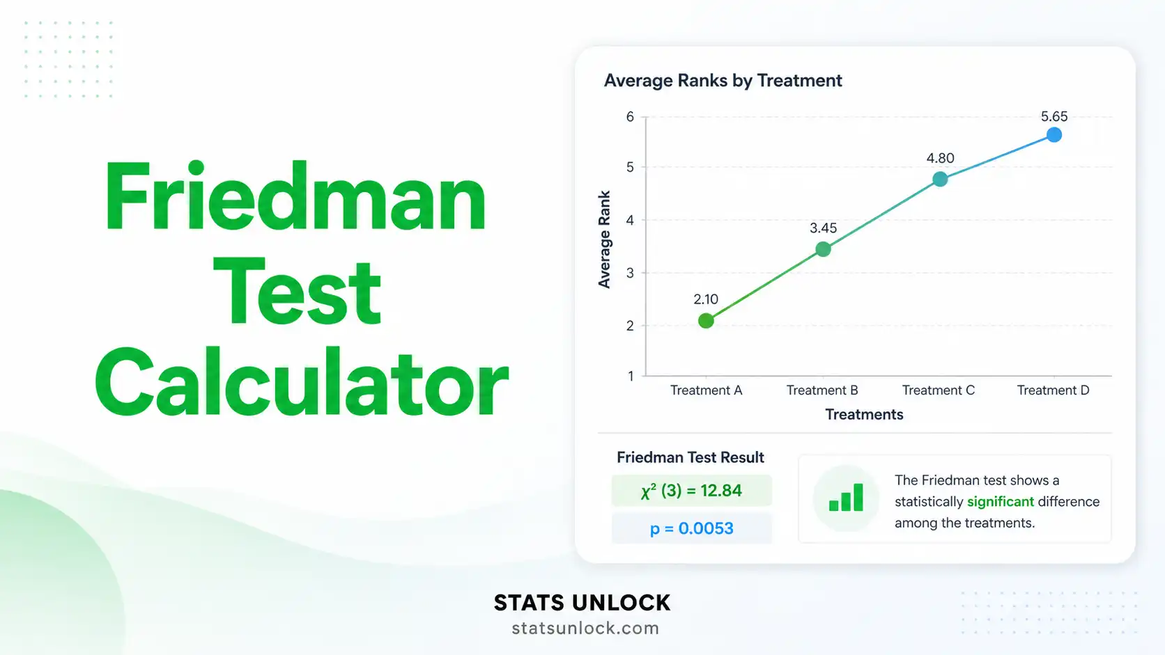
7. STEP 7 — Examine the two charts. The box plot shows the raw distribution per condition; the bar chart shows mean ranks. A significant Friedman test corresponds to visibly different mean ranks across bars.
8. STEP 8 — Check the assumption panel. Verifies sample size, equal-n requirement, and tie status with green/yellow/red badges.
9. STEP 9 — Read the interpretation. Section 6 auto-fills five paragraphs (plain-language interpretation) and five APA reporting templates.
10. STEP 10 — Export. Download Doc (.txt) for plain text; Download PDF for a print-formatted report; Copy summary for a one-line APA string.

The following references support the statistical methods used in this Friedman test calculator, covering nonparametric hypothesis testing, effect-size interpretation (Kendall's W), and APA-format reporting for repeated-measures research.

1. Friedman, M. (1937). The use of ranks to avoid the assumption of normality implicit in the analysis of variance. Journal of the American Statistical Association, 32(200), 675–701. https://doi.org/10.1080/01621459.1937.10503522
2. Friedman, M. (1940). A comparison of alternative tests of significance for the problem of m rankings. Annals of Mathematical Statistics, 11(1), 86–92. https://doi.org/10.1214/aoms/1177731944
3. Kendall, M. G., & Babington Smith, B. (1939). The problem of m rankings. Annals of Mathematical Statistics, 10(3), 275–287. https://doi.org/10.1214/aoms/1177732186
4. Conover, W. J. (1999). Practical Nonparametric Statistics (3rd ed.). John Wiley & Sons.
5. Nemenyi, P. B. (1963). Distribution-free multiple comparisons [Doctoral dissertation, Princeton University].
6. Cohen, J. (1988). Statistical power analysis for the behavioral sciences (2nd ed.). Lawrence Erlbaum Associates.
7. Field, A. (2018). Discovering statistics using IBM SPSS statistics (5th ed.). SAGE Publications.
8. Sheskin, D. J. (2011). Handbook of parametric and nonparametric statistical procedures (5th ed.). Chapman & Hall/CRC.
9. Pereira, D. G., Afonso, A., & Medeiros, F. M. (2015). Overview of Friedman's test and post-hoc analysis. Communications in Statistics — Simulation and Computation, 44(10), 2636–2653. https://doi.org/10.1080/03610918.2014.931971
10. Demšar, J. (2006). Statistical comparisons of classifiers over multiple data sets. Journal of Machine Learning Research, 7, 1–30. https://www.jmlr.org/papers/v7/demsar06a.html
11. American Psychological Association. (2020). Publication manual of the American Psychological Association (7th ed.). APA. https://doi.org/10.1037/0000165-000
12. Tomczak, M., & Tomczak, E. (2014). The need to report effect size estimates revisited. An overview of some recommended measures of effect size. Trends in Sport Sciences, 1(21), 19–25.
13. R Core Team. (2024). R: A language and environment for statistical computing. R Foundation for Statistical Computing. https://www.R-project.org/
14. Virtanen, P., Gommers, R., Oliphant, T. E., et al. (2020). SciPy 1.0: Fundamental algorithms for scientific computing in Python. Nature Methods, 17, 261–272. https://doi.org/10.1038/s41592-020-0772-5
15. NIST/SEMATECH. (2013). e-Handbook of Statistical Methods. National Institute of Standards and Technology. https://www.itl.nist.gov/div898/handbook/