What does statistical significance mean in a chi-square test?

Statistical significance (p < alpha) means your data are inconsistent with the null hypothesis of independence — the variables appear to be associated. It does NOT mean the association is strong or practically important. A huge sample can produce a statistically significant chi-square for a tiny, trivially weak association. Always report Cramér's V alongside the p-value to judge practical importance.

What is Cramér's V and how do I interpret it?

Cramér's V is the effect size for the chi-square test of independence. It ranges from 0 (no association) to 1 (perfect association). Cohen's (1988) benchmarks adjusted for table size: for a 2×2 table, V 0.50 = large. For larger tables, the same general direction applies but benchmarks shift slightly. Always report V alongside chi-square and p-value.

How large a sample do I need for a chi-square test of independence?

A general rule is that at least 80% of expected cell frequencies must be ≥ 5, and none should be < 1. For a 2×2 table detecting a medium effect (V = 0.30) at α = 0.05 with 80% power, you need approximately 88 participants. For larger tables, sample size requirements increase. Use the expected frequency table in this calculator to verify your sample is adequate before running the test.

What is the difference between one-tailed and two-tailed chi-square tests?

The chi-square test of independence is always one-tailed because the chi-square distribution is right-skewed and only large positive values indicate association. There is no concept of directionality — you are testing whether any association exists, not whether one variable is higher or lower than another. The p-value from the chi-square distribution is always the right-tail probability.

Chi-Square Test of Independence Calculator – Free Online Tool | Cramér’s V & p-Value

Chi-Square Test of Independence Calculator – Free Online Tool | Cramér's V & p-Value

📊 Step 1 — Enter Your Data

📦 Sample Dataset:

Enter observed frequencies row by row. Each row represents one category of your first variable. Separate values in a row with commas. Each row is a new line.

Variable 1 Name (Rows):

Variable 2 Name (Columns):

Row Category Labels (comma-separated): Column Category Labels (comma-separated): Observed Frequencies (one row per line, comma-separated):

Format: each line = one row category. Values = counts for each column category. E.g., "52, 48" means 52 in first column, 48 in second column for that row.

Upload CSV or Excel file (.csv, .txt, .xlsx, .xls):

Supports .csv, .txt, .xlsx, .xls — headers detected automatically. Click columns that should each become a row of the contingency table.

Rows: Columns:

⚙️ Step 2 — Test Configuration

Significance Level (α):

Yates' Continuity Correction:

Show Expected Frequencies:

📈 Results Summary

Statistic	Value	Description

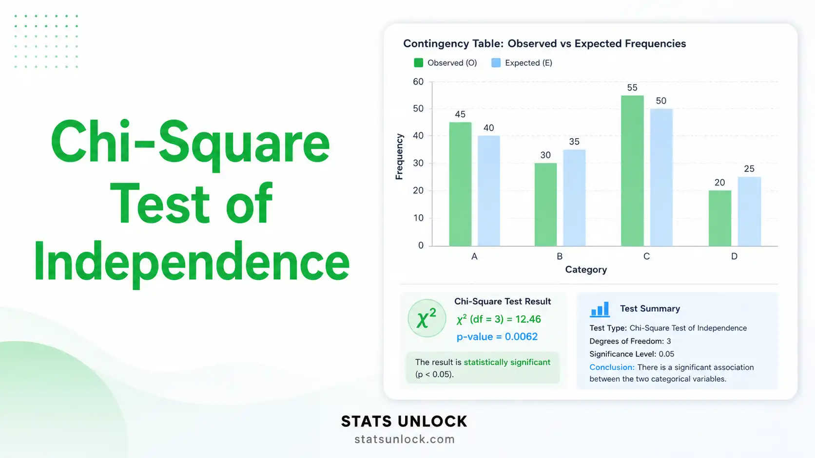
🔢 Observed vs Expected Frequencies

📊 Visualizations

📊 Observed vs Expected — by Row Category

🥧 χ² Contribution by Cell (% of Total)

📈 χ² Distribution — Acceptance & Rejection Regions

↔ Standardised Residuals — Diverging Bars

✅ Assumption Checks

🧠 Interpretation of Results

✍️ How to Write Your Results in Research

📋 Copy Summary to Clipboard

🔢 Technical Notes & Formulas

A. Formulas Used

1. Chi-Square Test Statistic (Standard)

χ² = Σ [(O_ij − E_ij)² / E_ij]

Where:
O_ij = observed frequency in row i, column j
E_ij = expected frequency in row i, column j
Σ = sum over all cells in the table
χ² = chi-square statistic (always ≥ 0; larger values = more deviation from independence)

2. Expected Frequency for Each Cell

E_ij = (Row_i Total × Column_j Total) / Grand Total (N)

Where:
Row_i Total = sum of all observed counts in row i
Column_j Total = sum of all observed counts in column j
N = total number of observations
E_ij = the frequency expected under the null hypothesis of independence

3. Degrees of Freedom

df = (r − 1) × (c − 1)

Where:
r = number of rows in the contingency table
c = number of columns in the contingency table
df = degrees of freedom used to find the p-value from the χ² distribution

4. Yates' Continuity Correction (2×2 only)

χ²_Yates = Σ [(|O_ij − E_ij| − 0.5)² / E_ij]

Where:
|O_ij − E_ij| = absolute difference between observed and expected
0.5 = Yates' correction factor, which reduces the test statistic slightly
Applied only for 2×2 tables; reduces Type I error rate for small samples

5. Cramér's V (Effect Size)

V = √(χ² / (N × min(r−1, c−1)))

Where:
χ² = the chi-square test statistic
N = total number of observations
min(r−1, c−1) = smaller of (rows−1) or (columns−1)
V = Cramér's V effect size; ranges 0 (no association) to 1 (perfect association)

6. Phi Coefficient (2×2 tables only)

φ = √(χ² / N)

Where:
χ² = chi-square statistic
N = total sample size
φ = phi coefficient; equivalent to Cramér's V for 2×2 tables; ranges 0 to 1

7. Standardised (Pearson) Residuals

r_ij = (O_ij − E_ij) / √E_ij

Where:
O_ij = observed count in cell (i,j)
E_ij = expected count in cell (i,j)
r_ij = standardised residual; values beyond ±2 indicate cells driving the association

8. Adjusted Standardised Residuals

d_ij = (O_ij − E_ij) / √[E_ij × (1 − R_i/N) × (1 − C_j/N)]

Where:
R_i = row i marginal total
C_j = column j marginal total
N = grand total
d_ij = adjusted standardised residual; approximately N(0,1); |d_ij| > 1.96 significant at α=.05

B. Technical Notes

The chi-square test of independence tests H₀: the two categorical variables are statistically independent (i.e., no association). H₁: the variables are associated (dependent).
The test is always one-tailed (right tail) because the chi-square distribution is non-negative and only large values suggest deviation from independence.
Yates' correction reduces the chi-square value slightly. It is recommended only for 2×2 tables with small expected cell counts; for larger tables or adequate samples it is controversial.
If the minimum expected cell frequency assumption is violated (any cell < 5), use Fisher's Exact Test (2×2) or consider collapsing categories.
Cramér's V is preferred over Phi for tables larger than 2×2. For 2×2, they are equivalent.
Standardised residuals identify which specific cells are responsible for the overall association. They are especially useful when interpreting larger tables.
The chi-square test does not indicate the direction of the association — it only detects whether one exists. Follow-up with residuals or proportional analyses to describe the direction.

📌 When to Use the Chi-Square Test of Independence

This free chi-square test of independence calculator is designed for researchers, students, and analysts who need to test whether two categorical variables are related. You use it whenever you have count data arranged in a contingency table and you want to know whether the distribution of one variable differs across levels of the other.

✅ Use the Chi-Square Test When:

✔ You have two categorical variables (nominal or ordinal)
✔ Each observation is independent — each person/unit appears in exactly one cell
✔ Your data are in the form of counts (frequencies), not means or proportions
✔ At least 80% of expected cell frequencies are ≥ 5 and none are < 1
✔ You want to know if knowing one variable predicts category membership in the other
✗ Do NOT use if your outcome variable is continuous — use t-test or ANOVA instead
✗ Do NOT use if observations are paired or matched — use McNemar's Test instead
✗ Do NOT use for small tables with expected cell counts < 5 — use Fisher's Exact Test
✗ Do NOT use if testing distribution fit against a theoretical model — use Chi-Square Goodness of Fit

🌍 Real-World Examples

🏥 Medical Research Is there an association between smoking status (smoker/non-smoker) and the presence of lung disease (yes/no) in a sample of 200 hospital patients?

🎓 Education Does teaching method (traditional lecture vs. flipped classroom) affect exam outcome (pass/fail) in a cohort of 150 university students?

📊 Marketing Is gender (male/female/non-binary) associated with brand preference (Brand A / B / C) in a consumer survey of 300 respondents?

🌿 Ecology Is habitat type (forest/grassland/wetland) associated with the presence or absence of a focal species across 120 surveyed sites?

🗺️ Decision Tree

Two Categorical Variables?
├─ Yes, Independent Observations → CHI-SQUARE TEST OF INDEPENDENCE ← (this tool)
│    ├─ 2×2 table, expected < 5 → Fisher's Exact Test
│    └─ Ordered categories → Linear-by-Linear Association (Mantel-Haenszel)
├─ Yes, Paired/Matched Data → McNemar's Test
└─ Testing fit to known distribution → Chi-Square Goodness of Fit Test

Continuous Outcome?
├─ Two groups → Independent t-Test / Mann-Whitney U
└─ 3+ groups → One-Way ANOVA / Kruskal-Wallis

📖 How to Use This Chi-Square Test of Independence Calculator — Step-by-Step Guide

Choose an input method. Use the three tabs at the top: (1) Paste/Type — enter frequencies as comma-separated rows; (2) Upload CSV/Excel — load a file and select which columns form each row of your table; (3) Contingency Grid — directly type counts into a visual table.
Try a sample dataset first. Click the "Sample Dataset" dropdown and select one of the five built-in examples (medical, education, marketing, ecology, politics). This loads real observed frequencies so you can see exactly how the tool works before entering your own data. The default sample is Smoking × Lung Disease.
Name your variables and categories. Enter your variable names (e.g., "Treatment Group" and "Recovery Status") and category labels (e.g., "Drug, Placebo" and "Recovered, Not Recovered"). Editable labels automatically appear in all charts, tables, and write-up templates.
Enter your observed frequencies. Each line in the text area represents one row category. Values on each line are comma-separated counts for each column category. For example, if 52 smokers have lung disease and 48 do not, the first line is "52, 48". Make sure row and column counts match your labels.
Configure test settings. Choose your alpha level (default 0.05). For 2×2 tables, decide whether to apply Yates' continuity correction — "Auto" applies it only when the table is 2×2. Toggle the expected frequencies display on or off.
Click "Run Chi-Square Analysis." The calculator instantly computes the χ² statistic, degrees of freedom, p-value, Cramér's V effect size, Phi (for 2×2), all expected frequencies, and standardised residuals for every cell.
Read the Summary Cards. Six cards show the most important values at a glance. Green = statistically significant; amber = borderline; red = not significant. Check the Cramér's V card to understand the strength of any association found.
Examine the four visualizations. (1) Grouped bar chart comparing observed vs expected counts; (2) contribution heatmap showing which cells deviate most from independence; (3) chi-square distribution curve with your test statistic and critical region shaded; (4) standardised residuals bar chart identifying which cells drive the association.
Check the assumption panel. Green badges mean the assumption is met; amber warnings mean the assumption is borderline and you should check carefully; red badges mean the assumption is violated. If minimum expected frequency is violated, switch to Fisher's Exact Test for 2×2 tables.
Copy a write-up template. Scroll to "How to Write Your Results in Research" for five auto-filled reporting templates. Click the green "📋 Copy" button next to the style you need (APA 7th, Thesis, Plain Language, Abstract, Pre-Registration). Download the full report as .txt or PDF using the buttons below the results.

❓ Frequently Asked Questions

Q1. What is the chi-square test of independence and when should I use it?

The chi-square test of independence tests whether two categorical variables are statistically associated or independent. It answers the question: "Does knowing a person's category on Variable A tell you anything about which category they fall into on Variable B?" You use it whenever you have count data in a contingency table — for example, testing whether smoking status (smoker/non-smoker) is related to the presence of lung disease (yes/no) in a group of hospital patients, or whether political party affiliation is associated with voting behaviour across different regions.

The test is non-parametric, meaning it does not assume your data are normally distributed. However, it does require that each observation is independent — each person or unit should appear in only one cell of the table.

Q2. What is a p-value in the chi-square test of independence, and how do I read it?

The p-value tells you the probability of observing a chi-square statistic as large as the one you calculated (or even larger), purely by chance, if the two variables were truly independent in the population. A small p-value (typically p < 0.05) means your result is unlikely to have occurred by chance alone, so you reject the null hypothesis of independence.

A common misconception is that the p-value equals the probability that the null hypothesis is true. It does not. The p-value describes how surprising your data are under the assumption that H₀ is true — not the probability that H₀ is correct. Always pair the p-value with an effect size (Cramér's V) to judge whether the association is meaningful, not just statistically detectable.

Q3. What does statistical significance mean — and does it equal practical importance?

Statistical significance (p < α) simply means your data are inconsistent with the null hypothesis of independence at your chosen alpha level. It does NOT mean the association is strong, large, or practically important. With a very large sample size, even a tiny, almost meaningless association can produce a statistically significant chi-square value because the test has enough power to detect trivially small deviations from independence.

This is why you must always report Cramér's V alongside the chi-square statistic. If Cramér's V is 0.05, the association is negligible in the real world — even if p < 0.001. Conversely, a non-significant result in a small sample may still reflect a real but undetected association. Statistical significance tells you about the reliability of your evidence, not the magnitude of the effect.

Q4. What is Cramér's V and how do I interpret the effect size benchmarks?

Cramér's V is the standard effect size measure for the chi-square test of independence. It ranges from 0 (the two variables are completely independent — knowing one tells you nothing about the other) to 1 (perfect association — knowing one variable perfectly predicts the other). For a 2×2 contingency table, Cramér's V equals the Phi coefficient.

Cohen's (1988) benchmarks, adjusted for table dimensions, provide practical interpretation guidelines. For a 2×2 table: V = 0.10 is a small effect, V = 0.30 is a medium effect, and V = 0.50 is a large effect. For larger tables (e.g., 3×3), the benchmarks shift slightly downward. A medium effect of V = 0.30 in a 2×2 table means the two variables share about 9% of their variance — a difference that is visible in real-world data and likely clinically or practically meaningful.

Q5. What are the assumptions of the chi-square test of independence, and what if they are violated?

The chi-square test of independence requires three key assumptions: (1) The two variables must be categorical (nominal or ordinal). (2) Observations must be independent — each participant or observation unit must appear in exactly one cell of the contingency table. (3) Expected cell frequencies must be adequate — at least 80% of cells must have an expected frequency of 5 or more, and no cell should have an expected frequency less than 1.

If the minimum expected frequency assumption is violated (typically due to a small total sample or rare categories), the chi-square approximation becomes unreliable. The recommended solutions are: use Fisher's Exact Test for 2×2 tables, collapse adjacent categories to increase cell counts, or collect more data. If observations are paired (e.g., before-and-after outcomes for the same people), use McNemar's Test instead.

Q6. How large a sample do I need for a reliable chi-square test of independence?

The key rule is that at least 80% of your expected cell frequencies must be 5 or greater, and no expected cell should be less than 1. This is not a fixed number of total participants — it depends on your table dimensions and the marginal distribution of your variables.

For a practical guide: a 2×2 table with roughly equal marginal distributions can produce adequate expected frequencies with as few as 20 total observations. However, for 80% power to detect a medium association (V = 0.30) at α = 0.05 in a 2×2 table, you typically need around 88 participants. For a 3×3 table with the same power requirements, you need approximately 200. Check the expected frequency table in this calculator to verify your sample meets the minimum requirement before interpreting results.

Q7. Why is the chi-square test always one-tailed? Can I do a one-tailed test for direction?

The chi-square test of independence is always one-tailed (right tail) because the chi-square statistic is always non-negative — it is a sum of squared quantities divided by expected values. The test asks whether the observed frequencies deviate from expected frequencies under independence, and any deviation in any direction produces a positive chi-square value. There is no concept of "left-tail" or "two-tailed" for this test in the traditional sense.

If you want to test for a specific directional relationship between two ordinal variables (e.g., higher income → higher education level), use the Mantel-Haenszel linear-by-linear association test or Spearman's rank correlation instead. The chi-square test does not tell you the direction of an association — it only tells you whether one exists. To understand direction, examine the standardised residuals or compare row/column percentages after obtaining a significant chi-square result.

Q8. How do I report chi-square test of independence results in APA 7th edition format?

The standard APA 7th edition format includes: the chi-square symbol (χ²), degrees of freedom, total N, the test statistic value, the p-value, and an effect size. Example: "A chi-square test of independence revealed a statistically significant association between smoking status and lung disease, χ²(1, N = 200) = 12.45, p < .001, Cramér's V = .25." Key rules: always italicise χ² and p; report p values to three decimal places; if p < .001, write "p < .001" (never "p = .000"); include N inside the parentheses after df; and always include Cramér's V — omitting effect size is an APA violation.

Scroll up to the "How to Write Your Results in Research" section on this page for five fully auto-filled reporting templates tailored to your specific data, covering APA 7th, thesis, plain-language, abstract, and pre-registration styles.

Q9. Can I use this chi-square calculator for published research or university assignments?

This calculator is designed for educational use, student coursework, and exploratory data analysis. The statistical algorithms are accurate and the results match those produced by R (chisq.test()), Python's scipy.stats.chi2_contingency(), SPSS, and SAS. However, for peer-reviewed journal submissions or formal research reports, we recommend verifying key results with established statistical software so you can specify the exact software and version used in your Methods section.

To cite this tool in your work: STATS UNLOCK. (2025). Chi-square test of independence calculator. Retrieved from https://statsunlock.com/chi-square-test-of-independence-calculator. Always verify with peer-reviewed statistical software for formal publication.

Q10. What should I do if my chi-square test result is non-significant — does it mean no association exists?

A non-significant result (p > α) means the data do not provide sufficient statistical evidence to reject the null hypothesis of independence. It does NOT prove that the variables are unrelated — it simply means the observed deviation from independence could plausibly have occurred by chance at your sample size. The two most common reasons for a non-significant result when a real association does exist are: insufficient statistical power (sample too small) and a genuinely weak effect that requires a very large sample to detect reliably.

If you expect an association but find a non-significant result, check your expected cell frequencies for assumption violations, compute a power analysis to see how large a sample would be needed to detect your expected effect size at 80% power, and report Cramér's V alongside the p-value so readers can judge the magnitude of the association for themselves. A Bayesian analysis with a Bayes Factor can help you quantify evidence in favour of independence rather than merely failing to reject it.

📚 References

The following peer-reviewed references support the chi-square test of independence calculator, including the statistical theory, effect size measures, assumption guidelines, and APA 7th edition reporting standards used in this hypothesis testing tool.

Pearson, K. (1900). On the criterion that a given system of deviations from the probable in the case of a correlated system of variables is such that it can be reasonably supposed to have arisen from random sampling. Philosophical Magazine, 50(302), 157–175. https://doi.org/10.1080/14786440009463897
Cohen, J. (1988). Statistical power analysis for the behavioral sciences (2nd ed.). Lawrence Erlbaum Associates. https://doi.org/10.4324/9780203771587
Cramér, H. (1946). Mathematical methods of statistics. Princeton University Press. https://press.princeton.edu/books/paperback/9780691005478
Agresti, A. (2013). Categorical data analysis (3rd ed.). Wiley. https://doi.org/10.1002/0471249688
Yates, F. (1934). Contingency tables involving small numbers and the χ² test. Supplement to the Journal of the Royal Statistical Society, 1(2), 217–235. https://doi.org/10.2307/2983604
Fisher, R. A. (1922). On the interpretation of χ² from contingency tables, and the calculation of P. Journal of the Royal Statistical Society, 85(1), 87–94. https://doi.org/10.2307/2340521
Cochran, W. G. (1952). The χ² test of goodness of fit. Annals of Mathematical Statistics, 23(3), 315–345. https://doi.org/10.1214/aoms/1177729380
American Psychological Association. (2020). Publication manual of the American Psychological Association (7th ed.). APA. https://doi.org/10.1037/0000165-000
Field, A. (2018). Discovering statistics using IBM SPSS statistics (5th ed.). SAGE Publications. https://uk.sagepub.com
Bergh, D. (2015). Chi-squared test of fit and sample size — A comparison between a random sample approach and a chi-squared approach. Journal of Applied Statistics, 42(3), 561–574. https://doi.org/10.1080/02664763.2014.963526
Tomczak, M., & Tomczak, E. (2014). The need to report effect size estimates revisited. An overview of some recommended measures of effect size. Trends in Sport Sciences, 1(21), 19–25. https://www.wbc.poznan.pl
Lakens, D. (2013). Calculating and reporting effect sizes to facilitate cumulative science: A practical primer for t-tests and ANOVAs. Frontiers in Psychology, 4, 863. https://doi.org/10.3389/fpsyg.2013.00863
Franke, T. M., Ho, T., & Christie, C. A. (2012). The chi-square test: Often used and more often misinterpreted. American Journal of Evaluation, 33(3), 448–458. https://doi.org/10.1177/1098214011426594
Rea, L. M., & Parker, R. A. (2014). Designing and conducting survey research: A comprehensive guide (4th ed.). Jossey-Bass. https://www.wiley.com
Virtanen, P., Gommers, R., Oliphant, T. E., et al. (2020). SciPy 1.0: Fundamental algorithms for scientific computing in Python. Nature Methods, 17, 261–272. https://doi.org/10.1038/s41592-020-0772-5