Pooled Standard Deviation Calculator
Paste comma-separated numbers for two or more groups, or upload a CSV, and get the pooled standard deviation instantly, together with the pooled variance, degrees of freedom, every group's own mean and SD, an equal-variance check, Cohen's d and Hedges' g, and full step-by-step working you can copy straight into a paper.
⚡ 0. Quick Answer
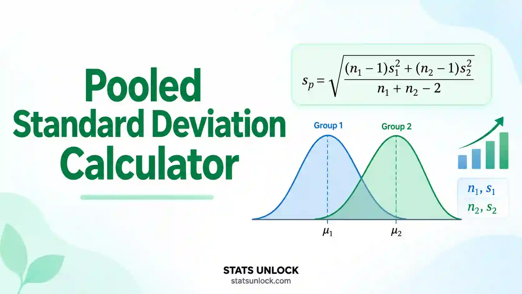
The pooled standard deviation is one combined estimate of spread built from two or more groups that are assumed to share the same true standard deviation.
You square each group's standard deviation, weight it by that group's degrees of freedom, add the weighted parts together, divide by the total degrees of freedom, and take the square root. For two groups of 12 with s₁ = 4.1960 and s₂ = 4.9013, the pooled variance is 20.8144 and the pooled standard deviation is 4.5623. It is the denominator of the two-sample t-test and of Cohen's d.
💡 Key Takeaways
- The pooled standard deviation weights each group by its degrees of freedom, nᵢ − 1, never by the raw sample size, so larger groups pull the answer more.
- You pool variances, not standard deviations. Averaging the SDs directly gives the wrong answer whenever the group sizes differ.
- The pooled degrees of freedom are N − k: total observations minus the number of groups. With two groups of 12 that is 22.
- Pooling assumes every group has the same true spread. As a working rule, stop pooling once the largest group variance is more than 4 times the smallest.
- The pooled SD always sits between the smallest and the largest group SD, and it is the denominator of both the two-sample t-test and Cohen's d.
- In one-way ANOVA the pooled standard deviation is exactly √MSwithin, the root mean square error from the ANOVA table.
📚 1. What Is Pooled Standard Deviation?
The pooled standard deviation is a single number that describes how spread out the observations are inside your groups, once every group has been combined into one estimate. It answers a narrow question: if all of these groups really do share the same underlying variability, and they only differ in where their centres sit, what is the best single estimate of that shared variability?
It is not the standard deviation of all the data thrown into one pile. That number would also contain the differences between the group means, which is exactly what you are usually trying to test. The pooled standard deviation strips those between-group differences out and keeps only the within-group scatter. That is why statisticians also call it the pooled within-group standard deviation or the pooled estimate of the common standard deviation.
How the pooling actually works, in four steps:
- Square each group's SD to get its variance. Variances add, standard deviations do not, so all pooling happens on the variance scale.
- Weight each variance by its degrees of freedom, nᵢ − 1. A group of 40 carries far more information about the common spread than a group of 5, and this weighting is what respects that.
- Add the weighted parts and divide by the total degrees of freedom, Σ(nᵢ − 1) = N − k. That gives the pooled variance, written sp².
- Take the square root to return to the original units. That is sp, the pooled SD.
A worked one-liner: two groups of 12 with standard deviations 4.1960 and 4.9013 have variances 17.6061 and 24.0227. Weighted by 11 degrees of freedom each, the pooled variance is (11 × 17.6061 + 11 × 24.0227) ÷ 22 = 20.8144, and the pooled standard deviation is 4.5623 with 22 degrees of freedom.
Who uses it: clinical trialists use it as the denominator of the two-sample t-test and of the standardised mean difference reported in every meta-analysis. Psychologists use it to build Cohen's d. Quality engineers use it to estimate short-term process variation across batches. Agronomists and ecologists meet it as the root mean square error in an ANOVA table, which is the same quantity under a different name. Anyone doing a power calculation needs it, because sample size formulas are written in units of the the pooled estimate.
| Quantity | What it measures | Use it when |
|---|---|---|
| Pooled standard deviation | Shared within-group spread, in original units | Groups plausibly share one true SD, and you need a t-test, Cohen's d or a power calculation |
| Pooled variance | The same thing squared, before the root | You are doing algebra, combining more terms, or reading MSwithin from an ANOVA table |
| Ordinary SD of all data combined | Total spread, within plus between groups | You want to describe the whole sample and are not comparing groups. It is not a substitute for sp |
| Each group's own SD | Spread inside one group only | You are describing groups separately, or checking whether pooling is even allowed |
| Welch standard error | Keeps the two variances separate | Group variances clearly differ, so pooling would be misleading |
🧮 2. Set Up Your Data
Type one value per cell. Each column becomes a group. Empty cells are ignored.
📊 3. Results
🧠 4. Interpretation of Results, In Detail
4.1 What does the pooled standard deviation actually tell you?
The pooled standard deviation tells you how far a typical observation sits from its own group's mean, once every group has been combined into one estimate. It is measured in the units of your data. It carries no information about how far apart the group means are, which is exactly what makes it a fair yardstick.
The pooled standard deviation is your best single answer to the question "how much do individual observations vary around their own group's mean?" It is expressed in the units of your data, so if you measured blood pressure in mmHg then sp is in mmHg, and you can read it the same way you read any standard deviation. A pooled SD of 4.56 mmHg means that within any group, a typical patient sits about 4.6 mmHg away from that group's mean.
What makes it different from an ordinary standard deviation is what it deliberately leaves out. It contains no information at all about how far apart the group means are. Two studies can share an identical pooled SD while one shows a huge treatment effect and the other shows none. That separation is the whole point: the pooled SD becomes the yardstick against which the difference between means is measured, and a yardstick must not itself depend on what you are measuring.
This is why almost every comparative statistic you meet has the pooled SD somewhere in its denominator. The t statistic divides the mean difference by a standard error built from sp. Cohen's d divides the same mean difference by sp itself. Sample size formulas are written in multiples of sp. Get the pooled SD wrong and every one of those numbers is wrong with it.
4.2 Why do you pool variances instead of averaging standard deviations?
Standard deviations are square roots, and square roots do not add. Squared deviations do add, so all combining has to happen on the variance scale, with one square root taken at the very end. Averaging two standard deviations of 2 and 8 gives 5, when the correct pooled answer is 5.83.
This is the single most common mistake, and it is worth being blunt about. Standard deviations are square roots, and square roots do not add. If you take the plain average of two standard deviations you are computing something that has no statistical meaning, and it will differ from the correct answer by an amount that grows as the groups become more different in size or spread.
The correct route is always the same. Square each SD to get a variance. Variances live on a scale where the weighted sum makes sense, because a variance is an average squared deviation and squared deviations genuinely add up. Combine on that scale, then take one square root at the very end.
Here is the size of the error. Two groups with SDs of 2 and 8 and equal sample sizes have a simple average of 5. The correct pooled value is the square root of (4 + 64) / 2, which is 5.83. That is a 17% understatement of the spread, and it will inflate every t statistic and every effect size you compute from it. When the sample sizes also differ, the gap widens further.
4.3 Why are the weights degrees of freedom rather than sample sizes?
Each group contributes n minus 1 rather than n because estimating that group's mean already consumed one piece of information. A group of one therefore gets a weight of zero, which is correct: it tells you nothing about spread. Larger groups dominate, because they genuinely carry more information about the common variability.
Each group contributes nᵢ − 1 to the pooled estimate rather than nᵢ. The reason is that you had to estimate the group's own mean before you could measure deviations from it, and that estimation consumes exactly one piece of information. A group of one tells you nothing about spread, and n − 1 correctly gives it a weight of zero.
The practical consequence is that larger groups dominate. A group of 100 carries 99 units of weight while a group of 10 carries 9, so the larger group influences the pooled value roughly eleven times as much. This is right and desirable: the bigger sample really does contain more information about the common spread. It also means that a small group with a wild standard deviation will move the pooled answer less than people expect, which is a feature rather than a bug.
It follows that the the pooled estimate always lies between the smallest and the largest group SD, never outside that range. If your calculator returns a value outside it, something has gone wrong with the input, usually a group entered twice or a sample size typed incorrectly.
4.4 What are the degrees of freedom for a pooled standard deviation?
The pooled degrees of freedom are N minus k: total observations minus the number of groups. Two groups of 12 give 24 minus 2 = 22. Four groups of 10 give 40 minus 4 = 36. Every group costs one degree of freedom because each one contributed its own mean to the calculation.
The pooled degrees of freedom are N − k, the total number of observations minus the number of groups. With two groups of 12 that is 24 − 2 = 22. With four groups of 10 it is 40 − 4 = 36. Every group costs you one degree of freedom because each one contributed its own mean.
Degrees of freedom matter for two reasons. They decide which t distribution you look the p value up in, and they tell you how much you should trust the pooled SD itself. Below about 10 pooled degrees of freedom the estimate is genuinely unstable and will bounce around noticeably from sample to sample. Above about 30 it settles down. Above 100 the t distribution is close enough to the normal that the distinction stops mattering in practice.
The df figure is also the fastest way to check that the tool and your software agree. If R reports df = 22 and your hand calculation says 23, you have miscounted a group somewhere, and the p values will not match until you fix it.
4.5 How equal do the group variances have to be before you can pool?
As a working rule, a variance ratio below 2 is comfortable, 2 to 4 is acceptable when the group sizes are similar, and above 4 you should stop pooling. Unequal group sizes make everything worse: a balanced design survives a ratio of 4, while a badly unbalanced one can fail at 2.
Pooling assumes homogeneity of variance: every group is drawn from a population with the same true standard deviation. If that holds, the pooled estimate is more precise than any single group's estimate, because it uses all the data. If it fails badly, the pooled value describes an average of two different things and misrepresents both.
The calculator gives you three ways to judge this. The variance ratio divides the largest group variance by the smallest. As a working rule, a ratio below 2 is comfortable, between 2 and 4 is acceptable when the group sizes are similar, and above 4 is a warning. The Levene style test, computed here on absolute deviations from each group's median and described in the NIST/SEMATECH e-Handbook of Statistical Methods, gives a formal p value: a small p value means the variances differ more than chance would explain. The chart of group variances lets you see whether one group is responsible or whether the spread rises steadily across groups.
Two important caveats. First, unequal group sizes make everything worse. With equal n, pooling is remarkably robust and survives a variance ratio of 3 or 4 without much damage. With very unequal n it can fail at a ratio of 2, and the direction of the error depends on whether the larger group is the more variable one. Second, a non-significant Levene test is not proof of equal variance, especially with small samples where the test has very little power. Use the ratio and the plot alongside it, not the p value alone.
4.6 What should you do when the variances are not equal?
Do not pool. Use Welch's t-test for two groups, or Welch's ANOVA with Games-Howell for more. If the spread grows with the mean, a log transformation often equalises the variances and lets you pool honestly on the transformed scale. Glass's delta avoids the assumption entirely by using the control group's SD.
Do not pool. The standard replacement for a two-group comparison is Welch's t-test, which keeps the two variances separate and adjusts the degrees of freedom downwards using the Welch-Satterthwaite formula. It costs almost nothing when the variances happen to be equal and protects you properly when they are not, which is why it is the default in R and why many methodologists now recommend using it always.
For more than two groups, Welch's ANOVA plays the same role, with the Games-Howell post hoc test in place of Tukey. If the spread rises with the mean, which is extremely common with counts, times and concentrations, a log or square root transformation will often make the variances equal and let you pool honestly on the transformed scale. Report the transformation and interpret on the transformed scale, or back-transform carefully.
If you still need an effect size when the variances differ, use Glass's delta, which divides by the control group's standard deviation alone rather than by a pooled value. It sidesteps the assumption entirely at the cost of using less of the data.
4.7 How is the pooled standard deviation used in Cohen's d?
Cohen's d divides the difference between two means by the pooled standard deviation, so a d of 1 means the means sit one pooled SD apart. Because the units cancel, d compares across studies. Hedges' g multiplies d by a correction factor J that removes the upward bias present in small samples.
Cohen's d is the difference between two means expressed in pooled standard deviations: d = (x̄₁ − x̄₂) ÷ sp. A d of 1 means the two means sit one pooled SD apart. Because it is unitless, it can be compared across studies that measured different things on different scales, which is exactly why meta-analysis depends on it.
The conventional bands are 0.2 small, 0.5 medium and 0.8 large, and they should be treated as very rough. Cohen himself proposed them reluctantly as a last resort for fields with no established benchmarks. In a well-controlled laboratory setting a d of 0.3 may be substantial; in a noisy field trial a d of 0.8 may be unremarkable. Where your discipline has typical effect sizes, use those instead.
Cohen's d is biased upward in small samples. Hedges' g applies a correction factor, J = 1 − 3 ÷ (4df − 1), which shrinks the estimate slightly. At df = 22 the correction is about 3.4%, at df = 10 it is about 7%, and above df = 50 it becomes negligible. Report g rather than d whenever your total sample is under about 20, and say which one you used either way, because reviewers cannot tell them apart from the number alone.
4.8 How does the pooled standard deviation build the two-sample t-test?
The standard error of the difference is the pooled SD multiplied by the square root of (1/n1 + 1/n2), and the t statistic is the mean difference divided by that standard error, on N minus 2 degrees of freedom. The same pieces build the confidence interval, so the two always agree.
The two-sample t-test with equal variances assumed uses the sp directly. The standard error of the difference is sp × √(1/n₁ + 1/n₂), and the t statistic is the mean difference divided by that. The degrees of freedom are the pooled df, n₁ + n₂ − 2.
The same pieces build the confidence interval for the difference: the mean difference plus or minus tcritical times that standard error. If the interval excludes zero, the test is significant at the matching alpha, and the two statements are guaranteed to agree because they are built from identical parts. Reporting the interval is more informative than reporting the p value alone, because it shows the range of differences your data are compatible with rather than just whether zero is in it.
Notice the role of the sample sizes here. The pooled SD describes the data and does not shrink as you collect more of it. The standard error does shrink, because of the 1/n terms. That distinction explains why a large study can find a tiny difference statistically significant while the pooled SD, and therefore the effect size, stays modest.
4.9 Is the pooled standard deviation the same as the root mean square error?
Yes, in one-way ANOVA. The mean square within groups is exactly the pooled variance, and its square root is exactly the pooled standard deviation. Software labels the same number root mean square error, residual standard error, or sigma. That means you can recover it from a published ANOVA table with no raw data.
In one-way ANOVA the mean square within groups, MSwithin, is exactly the pooled variance, and its square root is exactly the pooled standard deviation. Statistical software often labels it the root mean square error, RMSE, or the residual standard error. These are four names for one number.
That gives you a useful shortcut. If you already have an ANOVA table, you do not need the raw data to get the pooled SD: take the square root of the within-groups mean square. Conversely, if you have group means, SDs and sample sizes from a published paper, this calculator reconstructs the pooled SD and therefore the ANOVA error term without the original data, which is how meta-analysts work.
It also explains why Tukey's post hoc test uses the pooled SD from every group rather than just the two being compared. Using all the data gives more degrees of freedom and more power, provided the equal variance assumption holds across all groups, not just the pair in front of you.
4.10 How do you use the pooled standard deviation to plan sample size?
Power formulas are written in pooled SD units, so you need an estimate before collecting data. For a two-sample t-test at 80% power and alpha 0.05, you need roughly 16 divided by d squared participants per group. A d of 0.5 needs about 64 per group; a d of 0.8 needs about 25.
Power calculations are written in units of the the pooled value, which is why estimating it is normally the first step of a study design. For a two-sample t-test with 80% power at alpha = 0.05, you need roughly 16 ÷ d² participants per group, where d is the effect size you want to be able to detect. A d of 0.5 needs about 64 per group, and a d of 0.8 needs about 25.
The practical difficulty is that you need sp before you have collected the data. The usual sources are a pilot study, a published paper on a similar population, or a plausible range from which you compute sample size at the pessimistic end. Because sp from a small pilot is itself imprecise, it is sensible to use the upper end of its confidence interval rather than the point estimate, otherwise you will systematically design studies that are slightly too small.
4.11 A decision guide
| What you see | What it means | What to do |
|---|---|---|
| Variance ratio under 2, Levene p above 0.05 | Equal variances are plausible | Pool with confidence, use the pooled t-test and Cohen's d |
| Variance ratio 2 to 4, group sizes similar | Mild heterogeneity, low risk | Pooling is acceptable. Say so in the methods and note the ratio |
| Variance ratio 2 to 4, group sizes very unequal | Real risk of a wrong p value | Switch to Welch. Do not pool |
| Variance ratio above 4 | Groups do not share a common SD | Use Welch, or transform the data, or report Glass's delta |
| Spread grows with the group mean | Multiplicative rather than additive variation | Log transform, then re-check. Very common with counts and times |
| One group has a single extreme value | The variance ratio may be an artefact | Check chart 4, decide whether the point is genuine, and report either way |
| Pooled df under 10 | The pooled SD itself is unstable | Report it with a confidence interval and treat the effect size as provisional |
| A group has n = 1 | It contributes zero degrees of freedom | It cannot inform the pooled SD. Exclude it or collect more data |
4.12 Common mistakes this calculator prevents
- Averaging the standard deviations. The tool always squares first, weights by df, then takes one root at the end.
- Weighting by n instead of n − 1. The weights are shown explicitly in the working, so you can see them.
- Pooling the whole dataset. Computing one SD over all values combined includes the between-group differences and inflates the answer. The tool never does this and reports the total SD separately so you can see the gap.
- Using the population SD. The default is the n − 1 sample version, which is what the pooled formula requires.
- Ignoring unequal variances. The equal-variance panel runs automatically and flags a ratio above 4 in red.
- Reporting d when g was needed. Both are given, with the correction factor shown, so the small sample choice is explicit.
- Miscounting degrees of freedom. N, k and N − k are all displayed rather than assumed.
✍ 5. How to Write Your Results in Research
A pooled standard deviation is almost never the headline of a results section. It is the supporting number that makes the headline believable, so it usually appears inside a sentence about a t-test, an effect size or an ANOVA rather than on its own line. The five templates below cover the styles you are most likely to need. Each one is filled with your numbers once you press Calculate, and each has its own Copy button.
📌 Key conventions for this style
- APA italicises SD, M, t, p and d, but not the subscript p in sp.
- Report the exact p value to three decimals unless it is below .001.
- Always give the degrees of freedom in brackets after t.
- Give the effect size and its confidence interval, not just the p value.
- Say explicitly that equal variances were assumed, and name the test that justified it.
📌 Key conventions for this style
- State the formula in words, since an examiner wants to see that you know why variances are pooled and standard deviations are not.
- Report how homogeneity of variance was assessed and what the result was.
- Name the software and version, and say whether it defaults to Welch.
- Give every group's n, mean and SD in a table so the pooled value can be reproduced.
- Justify your choice of d or g explicitly by reference to the sample size.
📌 Key conventions for this style
- Never write sp, df, t or p in a plain-language summary.
- Say "how much people differed from each other" rather than "variance".
- Give the units every time a number appears.
- If the effect size is large, say what that means in the original units too.
📌 Key conventions for this style
- Declare the format once in the methods line and keep every row consistent.
- Abstracts have a word limit, so lead with the effect size and its interval, not the p value.
- Keep decimal places consistent down each column.
- Footnote whether the SD is the sample or population version.
📌 Key conventions for this style
- State in advance what you will do if the equal variance assumption fails, so the choice is not made after seeing the data.
- Give the assumed pooled SD used in the power calculation and where it came from.
- Pre-specify d or g, and whether the interval will be reported.
- Specify how outliers will be handled before the data are collected.
∑ 6. Formulas Used
📝 7. How Do You Use This Calculator?
- Enter your data. The default tab takes comma-separated numbers, exactly as the placeholder shows:
52, 48, 55, 61, 47, .... Newlines, tabs, semicolons and spaces all work, so a column pasted straight from Excel is fine. - Name each group. The group name box above every textarea is editable. Type something meaningful such as Placebo or Batch 3, night shift and it flows into the results table, all four charts and the exported report.
- Add or remove groups. Press Add group for a third, fourth or twelfth group. The pooled formula extends to any number of groups, and the degrees of freedom update to N − k automatically.
- Or upload a file. On the Upload tab, choose a CSV or Excel file and click the column names you want. Every column you click becomes its own group, and the preview highlights and badges the columns you have selected before you load them.
- Try a sample dataset. Ten built-in datasets cover the cases that matter: a clean clinical trial where pooling is exactly right, unequal group sizes, three and four group designs, a set where one group is far more variable than the others, and a case where a single outlier breaks the assumption.
- Keep the sample standard deviation setting. The n − 1 version is what the pooled formula is defined on. Only switch to the population version if you are deliberately reproducing a population calculation.
- Choose your confidence level and tails. These affect the confidence interval for the difference and the t-test p value when you have exactly two groups.
- Press Calculate Pooled Standard Deviation. Nothing is computed until you do, and changing any input or setting clears the results, so you never read stale numbers.
- Read the equal-variance panel before the headline number. The variance ratio and the Levene style test tell you whether pooling is defensible at all. A red flag there matters more than the pooled value itself.
- Check the four charts and export. Chart 1 shows every group mean against the pooled band, which is usually the figure you want in a paper. Section 5 auto-fills five reporting styles, and the buttons export a text report or a print-ready PDF.
Worked example. Load sample dataset 1, press Calculate, and you should see a pooled standard deviation of 4.5623 on 22 degrees of freedom, with Cohen's d = 1.8814 and Hedges' g = 1.8165. Those are the same numbers the Excel, R and Python sections below produce.
📈 8. How Do You Calculate Pooled Standard Deviation in Excel?
Excel has no POOLEDSD function, which is why this is one of the most searched spreadsheet questions in statistics. You build it from three functions you already know: VAR.S, COUNT and SQRT. This section shows the step by step layout first, because that is what a marker or a reviewer wants to see, then collapses the whole thing into a single cell formula, then extends it to three or more groups. Every screenshot uses the same worked dataset as the R and Python sections below, so all three agree to four decimal places.
=SQRT((VAR.S(A2:A13)*(COUNT(A2:A13)-1)+VAR.S(B2:B13)*(COUNT(B2:B13)-1))/(COUNT(A2:A13)+COUNT(B2:B13)-2)) and press Enter. That is the pooled standard deviation, 4.5623 for this data.8.1 The functions you need
| You want | Excel function | Note |
|---|---|---|
| Sample variance of a group | =VAR.S(A2:A13) | The n minus 1 version. This is the one the pooled formula needs |
| Sample standard deviation | =STDEV.S(A2:A13) | Square root of VAR.S. Use either, they carry the same information |
| Population variance | =VAR.P(A2:A13) | The n version. Do not use this for pooling |
| Group size | =COUNT(A2:A13) | Use COUNT, not COUNTA, which would count the header text |
| Group mean | =AVERAGE(A2:A13) | Needed for the mean difference and Cohen's d |
| Square root | =SQRT(E6) | The final step, turning pooled variance into pooled SD |
| Sum of squares directly | =DEVSQ(A2:A13) | Gives (n minus 1) times the variance in one step. Very handy for pooling |
| Two-sample t-test, pooled | =T.TEST(A2:A13,B2:B13,2,2) | The last argument 2 means equal variances assumed, which is the pooled test |
| t critical value | =T.INV.2T(0.05,22) | For a 95% confidence interval on 22 degrees of freedom |
| Analysis ToolPak route | Data → Data Analysis → t-Test: Two-Sample Assuming Equal Variances | Must enable the add-in first: File → Options → Add-ins → Manage Excel Add-ins → Go → tick Analysis ToolPak |
DEVSQ(range) returns the sum of squared deviations from the mean, which is exactly (n minus 1) times the sample variance. So the pooled standard deviation for any number of groups collapses to =SQRT((DEVSQ(A2:A13)+DEVSQ(B2:B13)+DEVSQ(C2:C13))/(COUNT(A2:A13)+COUNT(B2:B13)+COUNT(C2:C13)-3)). Note the minus 3: it is minus k, the number of groups, not always minus 2.8.2 Step by step
1 Put each group in its own column
One column per group, with a text label in row 1. The columns do not need to be the same length, since the pooled formula handles unequal group sizes correctly on its own.
The 12 placebo values sit in A2:A13 and the 12 treatment values in B2:B13. Only the first eight rows are shown here.
2 Get n, the mean, the SD and the variance for each group
Build a small summary block off to the side. You need the variance for the pooling itself and the mean for the effect size, so compute both now.
=COUNT(A2:A13)=AVERAGE(A2:A13)=STDEV.S(A2:A13)=VAR.S(A2:A13)Placebo has n = 12, mean 52.8333, SD 4.1960 and variance 17.6061. Treatment has n = 12, mean 44.2500, SD 4.9013 and variance 24.0227.
3 Weight each variance by its degrees of freedom, then take one square root
This is the step people get wrong. Multiply each variance by n minus 1, add the products, divide by the total degrees of freedom, and only then take the square root.
=E2-1=E5*D2=(E4+F4)/(D2+D3)=SQRT(E6)The two weighted sums of squares are 193.6667 and 264.2500. Their total, 457.9167, divided by 22 degrees of freedom gives a pooled variance of 20.8144, and the square root is the pooled standard deviation, 4.5623.
4 Collapse it into one cell, and see what the wrong method gives
Once you trust the layout, the whole calculation fits in a single formula. It is worth putting the incorrect method beside it once, so you can see how much averaging the standard deviations costs you.
=SQRT((VAR.S(A2:A13)*11+VAR.S(B2:B13)*11)/22)=SQRT((DEVSQ(A2:A13)+DEVSQ(B2:B13))/(COUNT(A2:A13)+COUNT(B2:B13)-2))=AVERAGE(STDEV.S(A2:A13),STDEV.S(B2:B13))The step by step block and the one cell formula both give 4.5623. Averaging the two standard deviations gives 4.5486, which is close here only because the group sizes are equal and the SDs are similar. Change either of those and the gap widens sharply.
5 Use the pooled SD for the t-test and Cohen's d
The pooled SD is rarely the end point. Feed it straight into the standard error, the t statistic and the effect size.
=E3*SQRT(1/12+1/12)=(AVERAGE(A2:A13)-AVERAGE(B2:B13))/E4=T.TEST(A2:A13,B2:B13,2,2)=(AVERAGE(A2:A13)-AVERAGE(B2:B13))/$E$3The mean difference is 8.5833 and the standard error is 1.8625, giving t = 4.6084 on 22 degrees of freedom, p = 0.000137, and Cohen's d = 1.8814. T.TEST with the last argument set to 2 returns the same p value, which is a useful cross-check.
8.3 Three or more groups, and other awkward cases
The two-group formula is a special case. For k groups the denominator is N minus k, not N minus 2, and forgetting to change it is the most common Excel error in this area.
=SQRT((DEVSQ(A2:A13)+DEVSQ(B2:B13)+DEVSQ(C2:C13))/(COUNT(A2:A13)+COUNT(B2:B13)+COUNT(C2:C13)-3))
Unequal group sizes need no special handling as long as each range is correct. Give each column its own COUNT rather than typing 12 three times, otherwise a change in one group silently corrupts the answer.
=SQRT((DEVSQ(A2:A31)+DEVSQ(B2:B21))/(COUNT(A2:A31)+COUNT(B2:B21)-2))
Long format data, where one column holds the value and another holds the group label, is more common in real files. Compute each group's sum of squares with a conditional variance built from AVERAGEIF and SUMPRODUCT, or simply sort by group and use separate ranges, which is faster and far easier to check.
=SUMPRODUCT((B2:B100="Placebo")*(A2:A100-AVERAGEIF(B2:B100,"Placebo",A2:A100))^2)
That expression gives the sum of squares for one group directly from long format data. Divide the total of these by N minus k as usual.
If you only have published means, SDs and sample sizes, and no raw data at all, the pooled SD is still recoverable. Enter the SDs and the n values in two small columns and use =SQRT(SUMPRODUCT((B2:B4-1),(C2:C4)^2)/(SUM(B2:B4)-COUNT(B2:B4))), with n in column B and SD in column C. This is exactly how meta-analysts reconstruct effect sizes from papers.
8.4 Why your Excel answer might differ from R or Python
| Situation | What happens | Fix |
|---|---|---|
You used VAR.P or STDEV.P | Excel divides by n, so every variance is too small and the pooled SD is too small | Use VAR.S and STDEV.S. NumPy has the mirror image problem: it defaults to ddof = 0 |
| NumPy gives a different SD | np.std defaults to the population formula | Write np.std(x, ddof=1) to match STDEV.S and R's sd() |
R's t.test disagrees | R defaults to Welch, which does not pool at all | Pass var.equal = TRUE to get the pooled test that matches Excel's T.TEST with the last argument 2 |
SciPy's ttest_ind disagrees | SciPy defaults to the pooled Student test, the opposite default to R | That is the pooled test already. Pass equal_var=False only if you want Welch |
| Denominator used minus 2 with three groups | Degrees of freedom too high, pooled SD slightly too small | The denominator is N minus k. With three groups it is minus 3 |
| Blank cells inside a range | Excel ignores them, so n is smaller than you expected | Check each COUNT returns the number you intended before trusting the result |
| Numbers stored as text | Silently skipped, so the variance is computed on fewer values | Look for green triangles in the cell corners, then Convert to Number |
| You averaged the SDs | Answer is too small, and the error grows with unequal n | Always square first, weight by df, and take one root at the end |
| Tool | Group variance | Pooled SD | Pooled t-test |
|---|---|---|---|
| Excel | =VAR.S(rng) | =SQRT((DEVSQ(a)+DEVSQ(b))/(COUNT(a)+COUNT(b)-2)) | =T.TEST(a,b,2,2) |
| Google Sheets | =VAR(rng) | Same formula as Excel | =TTEST(a,b,2,2) |
| R | var(x) | sqrt(((n1-1)*var(x)+(n2-1)*var(y))/(n1+n2-2)) | t.test(x, y, var.equal = TRUE) |
| Python SciPy | np.var(x, ddof=1) | np.sqrt(((n1-1)*v1+(n2-1)*v2)/(n1+n2-2)) | ttest_ind(x, y) |
| Python Pingouin | df['c'].var() | pingouin.compute_effsize(..., eftype='cohen') uses it internally | pingouin.ttest(x, y, correction=False) |
| SPSS | Analyze → Compare Means → Independent-Samples T Test. The "Equal variances assumed" row is the pooled one | ||
8.5 Charting the pooled standard deviation in Excel
- Select your group names and their means.
- Insert → Charts → Clustered Column.
- Click the chart, press the + button, tick Error Bars, then More Options → Custom → Specify Value and point at a column holding the pooled SD repeated once per group.
- Using the pooled SD for every bar rather than each group's own SD is the honest choice when you have already assumed equal variances, and it makes the figure agree with the test you ran.
- State in the caption that the bars are the pooled standard deviation. An unlabelled error bar is grounds for revision at most journals.
- To show the assumption itself, plot each group's variance as a second chart. If one bar towers over the others, pooling was not appropriate and the figure says so at a glance.
Charts 1 and 2 in section 3 of this page draw both of these automatically, which is usually quicker than rebuilding them in Excel.
8.6 Excel errors you will probably hit
| Excel shows | Why | Fix |
|---|---|---|
#DIV/0! from VAR.S | The range has fewer than two numeric values | A group of one contributes no degrees of freedom and cannot be pooled |
#DIV/0! from the pooled formula | Total degrees of freedom came out as zero | Check every COUNT. Usually a range points at empty cells |
#NUM! from SQRT | The pooled variance came out negative | Almost always a minus sign in the wrong place, or n minus 1 typed as 1 minus n |
#VALUE! | Text or a unit symbol typed into a data cell | Strip units into a separate column and re-enter the number |
#N/A from T.TEST | The two ranges are different sizes and you asked for a paired test | The third argument is tails, the fourth is type. Use 2 for tails and 2 for equal-variance independent |
| Pooled SD looks too small | You averaged the standard deviations instead of pooling the variances | Square, weight, sum, divide, then take one square root |
| Pooled SD outside the range of group SDs | A range overlaps another, or a group was entered twice | The pooled SD must sit between the smallest and largest group SD. If it does not, the input is wrong |
| Answer differs from a colleague | Different denominators, or a different SD version | Compare the degrees of freedom first. That finds it immediately in almost every case |
| Green triangles in cell corners | Numbers stored as text and being skipped | Select the column, click the warning icon, Convert to Number |
📈 9. How Do You Calculate Pooled Standard Deviation in R?
R has no single pooled.sd() function in base, which surprises people, but the calculation is three lines once you have the group variances. The script below is complete and runnable. It computes the pooled standard deviation for any number of groups, runs the equal-variance check, produces Cohen's d and Hedges' g when there are exactly two groups, prints a plain-English verdict, and saves one 300 dpi figure. It uses base R only, so there is nothing to install.
Rscript. Change only the groups <- list(...) lines to use your own data.9.1 The complete script
R, base only, saves pooled_sd_plot.png
# ============================================================
# Pooled standard deviation, pooled variance, Cohen's d and
# the equal-variance t-test, with one publication-ready plot
# StatsUnlock - https://statsunlock.com/pooled-standard-deviation-calculator/
# Base R only. No packages to install.
# ============================================================

set.seed(42)   # only matters if you add simulation below

# ---- 1. Your data ------------------------------------------
# Replace with your own values, or read a CSV:
#   dat <- read.csv("data.csv")
#   groups <- split(dat$value, dat$group)
# Missing values are dropped below, so NAs are safe here.

groups <- list(
  "Placebo"   = c(52, 48, 55, 61, 47, 50, 58, 53, 49, 56, 51, 54),
  "Treatment" = c(44, 41, 50, 38, 47, 45, 52, 40, 43, 49, 36, 46)
)

units <- "mmHg"

# ---- 2. Per-group statistics -------------------------------
groups <- lapply(groups, function(v) v[!is.na(v)])

n_i    <- sapply(groups, length)
mean_i <- sapply(groups, mean)
sd_i   <- sapply(groups, sd)          # sd() always uses n - 1
var_i  <- sd_i^2
df_i   <- n_i - 1
ss_i   <- df_i * var_i                # sum of squares inside each group

# ---- 3. The pooled standard deviation ----------------------
# Pool the VARIANCES, weighted by degrees of freedom.
# Never average the standard deviations directly.

df_pooled <- sum(df_i)                # N - k
var_pooled <- sum(ss_i) / df_pooled
sd_pooled  <- sqrt(var_pooled)

N <- sum(n_i)
k <- length(groups)

cat("=== Per-group statistics ===\n")
print(data.frame(n = n_i, mean = round(mean_i, 4),
                 sd = round(sd_i, 4), variance = round(var_i, 4),
                 df = df_i, sum_sq = round(ss_i, 4)))

cat(sprintf("\nN = %d across k = %d groups\n", N, k))
cat(sprintf("Total sum of squares within groups = %.4f\n", sum(ss_i)))
cat(sprintf("Pooled degrees of freedom (N - k)  = %d\n", df_pooled))
cat(sprintf("Pooled variance                    = %.4f\n", var_pooled))
cat(sprintf("POOLED STANDARD DEVIATION          = %.4f %s\n", sd_pooled, units))

# ---- 4. Equal-variance check -------------------------------
ratio <- max(var_i) / min(var_i)
cat(sprintf("\nVariance ratio (largest / smallest) = %.4f\n", ratio))
cat(if (ratio < 2)      "Verdict: comfortable, pooling is safe\n"
    else if (ratio < 4) "Verdict: acceptable if group sizes are similar\n"
    else                "Verdict: STOP, variances differ too much to pool\n")

# Brown-Forsythe (median-centred Levene) test
z <- unlist(lapply(groups, function(v) abs(v - median(v))))
g <- factor(rep(names(groups), n_i))
lev <- summary(aov(z ~ g))[[1]]
cat(sprintf("Levene (Brown-Forsythe) F = %.4f, p = %.4f\n",
            lev$"F value"[1], lev$"Pr(>F)"[1]))

# ---- 5. Two-group extras: t-test, Cohen's d, Hedges' g -----
if (k == 2) {
  x <- groups[[1]]; y <- groups[[2]]
  diff_means <- mean_i[1] - mean_i[2]
  se_diff <- sd_pooled * sqrt(1/n_i[1] + 1/n_i[2])
  t_stat  <- diff_means / se_diff
  p_val   <- 2 * pt(-abs(t_stat), df_pooled)
  tcrit   <- qt(0.975, df_pooled)
  ci      <- diff_means + c(-1, 1) * tcrit * se_diff

  d <- diff_means / sd_pooled
  J <- 1 - 3 / (4 * df_pooled - 1)
  hedges_g <- d * J

  cat("\n=== Two-group comparison ===\n")
  cat(sprintf("Mean difference = %.4f %s\n", diff_means, units))
  cat(sprintf("SE of difference = %.4f\n", se_diff))
  cat(sprintf("t(%d) = %.4f, p = %.6f\n", df_pooled, t_stat, p_val))
  cat(sprintf("95%% CI for the difference: [%.4f, %.4f]\n", ci[1], ci[2]))
  cat(sprintf("Cohen's d = %.4f   Hedges' g = %.4f (J = %.4f)\n",
              d, hedges_g, J))

  # Cross-check against the built-in test.
  # NOTE: R defaults to Welch, so var.equal = TRUE is required
  # to reproduce the pooled result.
  print(t.test(x, y, var.equal = TRUE))

  size <- if (abs(d) < 0.2) "negligible" else
          if (abs(d) < 0.5) "small" else
          if (abs(d) < 0.8) "medium" else "large"
  cat(sprintf("\nPlain English: the groups differ by %.2f %s, which is %.2f pooled\n",
              abs(diff_means), units, abs(d)))
  cat(sprintf("standard deviations, a %s effect. %s\n", size,
      if (p_val < 0.05) "The difference is statistically significant."
      else "The difference is not statistically significant."))
}

# ---- 6. One figure, two stacked panels ---------------------
png("pooled_sd_plot.png", width = 2700, height = 1950, res = 300)
layout(matrix(c(1, 2), nrow = 2), heights = c(3, 2))
par(mar = c(4.2, 4.6, 3, 1.4))

cols <- c("#2563eb", "#ea580c", "#16a34a", "#9333ea",
          "#0d9488", "#c2410c")[seq_len(k)]

# Panel 1: group means with pooled SD bars
bp <- barplot(mean_i, names.arg = names(groups), col = cols,
              border = NA, ylim = c(0, max(mean_i + 2 * sd_pooled)),
              ylab = paste0("Mean (", units, ")"),
              main = sprintf("Group means with pooled SD bars (sp = %.4f)", sd_pooled))
arrows(bp, mean_i - sd_pooled, bp, mean_i + sd_pooled,
       angle = 90, code = 3, length = 0.06, lwd = 2)
text(bp, mean_i / 2, sprintf("%.2f", mean_i), col = "white", font = 2)

# Panel 2: each group's variance against the pooled variance
par(mar = c(4.2, 4.6, 3, 1.4))
barplot(var_i, names.arg = names(groups), col = "#cbd5e1", border = NA,
        ylab = "Variance", main = "Group variances vs pooled variance")
abline(h = var_pooled, col = "#dc2626", lwd = 2.5, lty = 2)
legend("topright", legend = sprintf("pooled variance = %.4f", var_pooled),
       col = "#dc2626", lty = 2, lwd = 2.5, bty = "n")

dev.off()
cat("\nFigure saved as pooled_sd_plot.png at 300 dpi\n")
9.2 What each part of the script does
| Block | What it does | Why it matters |
|---|---|---|
groups <- list(...) | Holds each group as a named vector | A named list extends to any number of groups with no other change to the script |
v[!is.na(v)] | Drops missing values | A single NA would turn every downstream statistic into NA |
sd_i <- sapply(groups, sd) | Group standard deviations | R's sd() always uses the n minus 1 denominator, which is what pooling needs |
ss_i <- df_i * var_i | Sum of squares inside each group | This is the quantity that actually gets added. Variances add, standard deviations do not |
df_pooled <- sum(df_i) | N minus k | Works automatically for two groups or twelve, unlike a hard-coded n1 + n2 minus 2 |
sqrt(sum(ss_i) / df_pooled) | The pooled SD itself | One square root, taken only at the very end |
ratio <- max(var_i)/min(var_i) | The variance ratio | The fastest check on whether pooling is defensible at all |
aov(z ~ g) on abs(v - median(v)) | Brown-Forsythe version of Levene's test | Median centring makes it robust to non-normal data, which the mean-centred version is not |
J <- 1 - 3/(4*df_pooled - 1) | Small-sample correction factor | Turns Cohen's d into Hedges' g. Always slightly below 1 |
t.test(x, y, var.equal = TRUE) | Cross-check against the built-in test | Essential. Without var.equal = TRUE R runs Welch and does not pool at all |
png(..., res = 300) | Opens a 300 dpi device | Journals reject screenshots. This writes a real print-quality file |
9.3 What the figure shows
The saved pooled_sd_plot.png has two stacked panels. The upper panel plots each group mean as a bar with error bars set to the pooled standard deviation rather than each group's own, which is the consistent choice once you have assumed a common spread. The lower panel plots each group's variance as a grey bar with the pooled variance drawn across as a red dashed line. If one grey bar towers over the red line while another sits far below it, the equal-variance assumption has failed and the figure says so without a single number.
Read the two panels together. The upper panel answers "how far apart are the groups?" and the lower panel answers "was I allowed to ask that question this way?".
9.4 Problems and fixes in R
| Symptom | Cause | Fix |
|---|---|---|
Your t and p do not match t.test | R defaults to Welch, which does not use the pooled SD, as the official t.test documentation states | Add var.equal = TRUE. This is the single most common R surprise in this area |
Everything returns NA | One missing value in a group | The script drops NAs already. If you bypass that, use sd(x, na.rm = TRUE) and recount n |
Error in split: ... | The grouping column is numeric, not a factor | Wrap it: factor(dat$group) |
| Pooled SD is smaller than every group SD | You averaged the SDs somewhere | Check you squared before summing. The pooled value must lie between the smallest and largest group SD |
| Levene test not found | car::leveneTest needs the car package | The script uses base aov on absolute median deviations, which is the same test with no dependency |
| Figure is blank | dev.off() was never reached because of an error above it | Run dev.off() manually, then rerun the block from the top |
| Groups of different lengths break your own code | You used a matrix or data frame instead of a list | A list handles ragged groups. A data frame forces equal lengths and pads with NA |
sapply returns a list not a vector | One group has zero elements after NA removal | Drop empty groups before the summary step |
9.5 One-liners worth remembering
| Task | R |
|---|---|
| Pooled SD, two groups | sqrt(((length(x)-1)*var(x) + (length(y)-1)*var(y)) / (length(x)+length(y)-2)) |
| Pooled SD, any number of groups | sqrt(sum(sapply(g, function(v) (length(v)-1)*var(v))) / (sum(lengths(g)) - length(g))) |
| Pooled SD from an ANOVA fit | sigma(aov(value ~ group, data = dat)) |
| Pooled SD from a linear model | summary(lm(value ~ group, data = dat))$sigma |
| Pooled t-test | t.test(x, y, var.equal = TRUE) |
| Cohen's d | effsize::cohen.d(x, y, pooled = TRUE) |
| Hedges' g | effsize::cohen.d(x, y, hedges.correction = TRUE) |
| Levene test with the car package | car::leveneTest(value ~ group, data = dat) |
| Bartlett test, normal data only | bartlett.test(value ~ group, data = dat) |
The sigma() one-liner is the quickest route of all. In one-way ANOVA the residual standard error is the pooled standard deviation, so fitting the model and reading sigma gives the same 4.5623 the long script produces.
📈 10. How Do You Calculate Pooled Standard Deviation in Python?
Python has one trap that catches almost everyone: NumPy's var and std default to the population formula, dividing by n rather than n minus 1. Pass ddof=1 every time and your answers will match R, Excel and this calculator exactly. The script below is complete and runnable, handles any number of groups, and saves one 300 dpi figure.
numpy for the arithmetic, scipy.stats for the t distribution and Levene's test, matplotlib for the figure. Install them once with pip install numpy scipy matplotlib. Pandas is optional and only needed for the commented CSV route.groups = {...} dictionary to use your own data.10.1 The complete script
Python 3, saves pooled_sd_plot.png
# ============================================================
# Pooled standard deviation, pooled variance, Cohen's d and
# the equal-variance t-test, with one publication-ready plot
# StatsUnlock - https://statsunlock.com/pooled-standard-deviation-calculator/
# pip install numpy scipy matplotlib
# ============================================================

import numpy as np
import matplotlib
matplotlib.use("Agg")
import matplotlib.pyplot as plt
from scipy import stats

np.random.seed(42)   # only matters if you add simulation below

# ---- 1. Your data ------------------------------------------
# Replace with your own values, or read a CSV:
#   import pandas as pd
#   df = pd.read_csv("data.csv")
#   groups = {g: sub["value"].dropna().to_numpy()
#             for g, sub in df.groupby("group")}

groups = {
    "Placebo":   np.array([52, 48, 55, 61, 47, 50, 58, 53, 49, 56, 51, 54], float),
    "Treatment": np.array([44, 41, 50, 38, 47, 45, 52, 40, 43, 49, 36, 46], float),
}

units = "mmHg"

# Drop missing values so NaNs never silently corrupt a variance.
groups = {g: v[~np.isnan(v)] for g, v in groups.items()}

# ---- 2. Per-group statistics -------------------------------
names = list(groups)
n_i    = np.array([len(groups[g]) for g in names])
mean_i = np.array([groups[g].mean() for g in names])
# ddof=1 is essential: NumPy defaults to the POPULATION formula.
var_i  = np.array([groups[g].var(ddof=1) for g in names])
sd_i   = np.sqrt(var_i)
df_i   = n_i - 1
ss_i   = df_i * var_i

# ---- 3. The pooled standard deviation ----------------------
# Pool the VARIANCES, weighted by degrees of freedom.
# Never average the standard deviations directly.

N, k = int(n_i.sum()), len(names)
df_pooled  = int(df_i.sum())          # N - k
var_pooled = ss_i.sum() / df_pooled
sd_pooled  = np.sqrt(var_pooled)

print("=== Per-group statistics ===")
print(f"{'group':<14}{'n':>5}{'mean':>12}{'sd':>12}{'variance':>12}{'df':>6}{'sum_sq':>12}")
for i, g in enumerate(names):
    print(f"{g:<14}{n_i[i]:>5}{mean_i[i]:>12.4f}{sd_i[i]:>12.4f}"
          f"{var_i[i]:>12.4f}{df_i[i]:>6}{ss_i[i]:>12.4f}")

print(f"\nN = {N} across k = {k} groups")
print(f"Total sum of squares within groups = {ss_i.sum():.4f}")
print(f"Pooled degrees of freedom (N - k)  = {df_pooled}")
print(f"Pooled variance                    = {var_pooled:.4f}")
print(f"POOLED STANDARD DEVIATION          = {sd_pooled:.4f} {units}")

# ---- 4. Equal-variance check -------------------------------
ratio = var_i.max() / var_i.min()
print(f"\nVariance ratio (largest / smallest) = {ratio:.4f}")
if ratio < 2:
    print("Verdict: comfortable, pooling is safe")
elif ratio < 4:
    print("Verdict: acceptable if group sizes are similar")
else:
    print("Verdict: STOP, variances differ too much to pool")

lev_F, lev_p = stats.levene(*[groups[g] for g in names], center="median")
print(f"Levene (Brown-Forsythe) F = {lev_F:.4f}, p = {lev_p:.4f}")

# ---- 5. Two-group extras: t-test, Cohen's d, Hedges' g -----
if k == 2:
    x, y = groups[names[0]], groups[names[1]]
    diff = mean_i[0] - mean_i[1]
    se_diff = sd_pooled * np.sqrt(1 / n_i[0] + 1 / n_i[1])
    t_stat = diff / se_diff
    p_val = 2 * stats.t.sf(abs(t_stat), df_pooled)
    tcrit = stats.t.ppf(0.975, df_pooled)
    ci = (diff - tcrit * se_diff, diff + tcrit * se_diff)

    d = diff / sd_pooled
    J = 1 - 3 / (4 * df_pooled - 1)
    g_hedges = d * J

    print("\n=== Two-group comparison ===")
    print(f"Mean difference  = {diff:.4f} {units}")
    print(f"SE of difference = {se_diff:.4f}")
    print(f"t({df_pooled}) = {t_stat:.4f}, p = {p_val:.6f}")
    print(f"95% CI for the difference: [{ci[0]:.4f}, {ci[1]:.4f}]")
    print(f"Cohen's d = {d:.4f}   Hedges' g = {g_hedges:.4f} (J = {J:.4f})")

    # Cross-check. NOTE: SciPy DEFAULTS to the pooled Student test,
    # the opposite default to R. Pass equal_var=False for Welch.
    print("SciPy check:", stats.ttest_ind(x, y, equal_var=True))

    size = ("negligible" if abs(d) < 0.2 else "small" if abs(d) < 0.5
            else "medium" if abs(d) < 0.8 else "large")
    verdict = ("statistically significant" if p_val < 0.05
               else "not statistically significant")
    print(f"\nPlain English: the groups differ by {abs(diff):.2f} {units}, which is "
          f"{abs(d):.2f} pooled standard deviations, a {size} effect. "
          f"The difference is {verdict}.")

# ---- 6. One figure, two stacked panels ---------------------
palette = ["#2563eb", "#ea580c", "#16a34a", "#9333ea", "#0d9488", "#c2410c"]
cols = [palette[i % len(palette)] for i in range(k)]

fig, ax = plt.subplots(2, 1, figsize=(9, 6.5), height_ratios=[3, 2])

ax[0].bar(names, mean_i, color=cols, yerr=sd_pooled, capsize=6,
          error_kw={"elinewidth": 2, "ecolor": "#334155"})
ax[0].set_ylabel(f"Mean ({units})")
ax[0].set_title(f"Group means with pooled SD bars (sp = {sd_pooled:.4f})")
for i, m in enumerate(mean_i):
    ax[0].text(i, m / 2, f"{m:.2f}", ha="center", color="white", fontweight="bold")

ax[1].bar(names, var_i, color="#cbd5e1")
ax[1].axhline(var_pooled, color="#dc2626", lw=2.5, ls="--",
              label=f"pooled variance = {var_pooled:.4f}")
ax[1].set_ylabel("Variance")
ax[1].set_title("Group variances vs pooled variance")
ax[1].legend(frameon=False)

for a in ax:
    a.spines[["top", "right"]].set_visible(False)

fig.tight_layout()
fig.savefig("pooled_sd_plot.png", dpi=300)
print("\nFigure saved as pooled_sd_plot.png at 300 dpi")
10.2 What each part of the script does
| Block | What it does | Why it matters |
|---|---|---|
matplotlib.use("Agg") | Selects a non-interactive backend | Lets the script run on a server or in CI with no display attached |
groups = {...} | A dictionary of name to array | Extends to any number of groups with no other change |
v[~np.isnan(v)] | Drops missing values | A single NaN propagates through every later statistic silently |
var(ddof=1) | Sample variance | The critical line. Without ddof=1 NumPy divides by n and your pooled SD is too small |
ss_i = df_i * var_i | Sum of squares inside each group | The quantity that is actually summed across groups |
df_pooled = int(df_i.sum()) | N minus k | Correct for any k, unlike a hard-coded n1 + n2 minus 2 |
np.sqrt(ss_i.sum()/df_pooled) | The the pooled estimate | One square root, at the very end |
stats.levene(..., center="median") | Brown-Forsythe test | The median-centred version is robust. SciPy's default is already median, but stating it makes the choice explicit |
stats.t.sf(abs(t), df) | Upper tail probability | More numerically accurate in the far tail than 1 - cdf |
ttest_ind(x, y, equal_var=True) | Cross-check | SciPy defaults to the pooled test, the opposite default to R. Stating it avoids confusion later |
fig.savefig(..., dpi=300) | Writes the figure | 300 dpi is the normal journal minimum for a raster figure |
10.3 What the figure shows
The same two panels as the R script, so the two outputs can be compared side by side. The upper panel shows the group means with pooled SD error bars, and the lower panel shows each group's variance against the pooled variance as a red dashed line. Matplotlib's capsize=6 puts caps on the error bars so they read clearly in print, and the top and right spines are removed because most journals prefer that style.
If you want each group's own SD on the error bars instead of the pooled value, replace yerr=sd_pooled with yerr=sd_i. Whichever you choose, say which one in the caption.
10.4 Problems and fixes in Python
| Symptom | Cause | Fix |
|---|---|---|
| Pooled SD slightly too small | NumPy used ddof=0, the population formula | Always write np.var(x, ddof=1) and np.std(x, ddof=1) |
Everything is nan | A NaN in one group | Filter with v[~np.isnan(v)], or use np.nanvar(x, ddof=1) |
| SciPy result differs from R | Different defaults: SciPy's ttest_ind pools, R uses Welch | Set the argument explicitly in both, then they agree exactly |
height_ratios raises TypeError | Matplotlib older than 3.6 | Use gridspec_kw={"height_ratios": [3, 2]} instead |
integer division surprises | Group sizes stored as Python ints in old code | Cast the arrays to float, as the script does with the float dtype argument |
| Figure never appears | The Agg backend writes to file and shows nothing | That is intended. Open pooled_sd_plot.png, or drop the use("Agg") line in a notebook |
| Pandas groupby gives a Series not an array | sub["value"] is a Series | Add .to_numpy(), as the commented CSV block does |
| Levene p value differs from SPSS | SPSS centres on the mean by default, SciPy on the median | Pass center="mean" to reproduce SPSS, but the median version is the more robust choice |
10.5 One-liners worth remembering
| Task | Python |
|---|---|
| Sample variance | np.var(x, ddof=1) |
| Pooled SD, two groups | np.sqrt(((len(x)-1)*x.var(ddof=1) + (len(y)-1)*y.var(ddof=1)) / (len(x)+len(y)-2)) |
| Pooled SD, any number of groups | np.sqrt(sum((len(v)-1)*v.var(ddof=1) for v in gs) / (sum(map(len, gs)) - len(gs))) |
| Pooled t-test | scipy.stats.ttest_ind(x, y, equal_var=True) |
| Welch t-test | scipy.stats.ttest_ind(x, y, equal_var=False) |
| Cohen's d with Pingouin | pingouin.compute_effsize(x, y, eftype="cohen") |
| Hedges' g with Pingouin | pingouin.compute_effsize(x, y, eftype="hedges") |
| Levene test | scipy.stats.levene(x, y, center="median") |
| Pooled SD from an OLS fit | np.sqrt(statsmodels.formula.api.ols("value ~ C(group)", d).fit().mse_resid) |
That last line is the Python mirror of R's sigma(): the residual mean square from a one-way model is the pooled variance, so its square root is the pooled standard deviation, 4.5623 for the worked dataset.
📋 11. Reference Tables
11.1 Degrees of freedom for common designs
| Design | N | k | Pooled df (N − k) | Note |
|---|---|---|---|---|
| Two groups of 10 | 20 | 2 | 18 | The classic small trial |
| Two groups of 12 | 24 | 2 | 22 | The worked example on this page |
| Two groups of 30 | 60 | 2 | 58 | t is close to z at this point |
| 20 controls and 8 treated | 28 | 2 | 26 | Unequal n needs no special handling |
| Three groups of 8 | 24 | 3 | 21 | Minus 3, not minus 2. The usual mistake |
| Four groups of 6 | 24 | 4 | 20 | Each group costs one df |
| Five groups of 20 | 100 | 5 | 95 | Very stable pooled estimate |
| Two groups, one with n = 1 | n+1 | 2 | n − 1 | The single observation contributes nothing |
Conclusion: subtract one degree of freedom per group, never a fixed 2. Check this figure against your software before comparing any p value.
11.2 t critical values at the pooled degrees of freedom
| df | 90% two-tailed | 95% two-tailed | 99% two-tailed |
|---|---|---|---|
| 4 | 2.132 | 2.776 | 4.604 |
| 8 | 1.860 | 2.306 | 3.355 |
| 10 | 1.812 | 2.228 | 3.169 |
| 18 | 1.734 | 2.101 | 2.878 |
| 20 | 1.725 | 2.086 | 2.845 |
| 22 | 1.717 | 2.074 | 2.819 |
| 30 | 1.697 | 2.042 | 2.750 |
| 60 | 1.671 | 2.000 | 2.660 |
| 120 | 1.658 | 1.980 | 2.617 |
| ∞ | 1.645 | 1.960 | 2.576 |
Conclusion: multiply the standard error by the value in the 95% column to build a confidence interval for the difference between means. Note how little changes above df = 30.
11.3 Variance ratio, and whether you may pool
| Largest ÷ smallest variance | Equal group sizes | Unequal group sizes | Verdict |
|---|---|---|---|
| 1.0 to 1.5 | Safe | Safe | Pool with confidence |
| 1.5 to 2.0 | Safe | Safe | Pool, mention the ratio in the methods |
| 2.0 to 3.0 | Acceptable | Caution | Pool only if the group sizes are close |
| 3.0 to 4.0 | Caution | Do not pool | Prefer Welch unless n is balanced and large |
| 4.0 to 9.0 | Do not pool | Do not pool | Welch, or transform the data first |
| Above 9.0 | Do not pool | Do not pool | The groups do not share a common SD at all |
Conclusion: balanced designs are far more forgiving than unbalanced ones. If you can choose your group sizes, make them equal, because that single decision buys you most of the robustness.
11.4 The Hedges' g correction factor J at each df
| Pooled df | J = 1 − 3 ÷ (4df − 1) | Shrinkage | Which to report |
|---|---|---|---|
| 4 | 0.8000 | 20.0% | Always g |
| 8 | 0.9032 | 9.7% | Always g |
| 10 | 0.9231 | 7.7% | Always g |
| 18 | 0.9577 | 4.2% | Prefer g |
| 22 | 0.9655 | 3.5% | Prefer g |
| 30 | 0.9748 | 2.5% | Either, state which |
| 50 | 0.9849 | 1.5% | Either, state which |
| 100 | 0.9925 | 0.8% | d is fine |
| 200 | 0.9962 | 0.4% | d is fine |
Conclusion: below about 20 degrees of freedom the correction is large enough to change how a result reads, so report Hedges' g. Above 100 it is invisible and the choice does not matter, but you should still say which one you used.
11.5 Effect size bands and what they mean in pooled SD units
| Cohen's d | Label | Overlap between the two distributions | Rough meaning |
|---|---|---|---|
| 0.0 | None | 100% | The groups are indistinguishable |
| 0.2 | Small | 85% | Detectable in a big study, invisible to the eye |
| 0.5 | Medium | 67% | Visible to a careful observer |
| 0.8 | Large | 53% | Obvious in a plot of the raw data |
| 1.2 | Very large | 38% | Rare outside strongly controlled settings |
| 2.0 | Huge | 19% | Check for a coding error or a ceiling effect first |
Conclusion: these bands are conventions, not laws. In a field with typical effect sizes of 0.15, a d of 0.4 is remarkable. Use your own literature as the benchmark where you can.
11.6 Sample size per group for a two-sample t-test
| Target Cohen's d | n per group, 80% power | n per group, 90% power | Total N at 80% |
|---|---|---|---|
| 0.2 | 394 | 527 | 788 |
| 0.3 | 176 | 235 | 352 |
| 0.4 | 100 | 133 | 200 |
| 0.5 | 64 | 86 | 128 |
| 0.6 | 45 | 60 | 90 |
| 0.8 | 26 | 34 | 52 |
| 1.0 | 17 | 23 | 34 |
| 1.2 | 12 | 16 | 24 |
Conclusion: two-tailed test at alpha = 0.05. Because d is the raw difference divided by the pooled standard deviation, you must estimate sp before you can use this table. A pilot study or a published paper on a similar population is the usual source.
11.7 Names for the same quantity across software and textbooks
| Name you will see | Where | Is it the pooled SD? |
|---|---|---|
| Pooled SD, sp | Textbooks, this page | Yes |
| Pooled estimate of the common standard deviation | Older texts, quality control | Yes |
| Pooled within-group standard deviation | Meta-analysis, psychology | Yes |
| Root mean square error, RMSE | ANOVA and regression output | Yes, in one-way ANOVA |
| Residual standard error | R's summary(lm) | Yes, in a one-way model |
| √MSwithin or √MSerror | ANOVA tables | Yes |
Sigma, sigma() | R model objects | Yes |
| Standard error of the difference | t-test output | No. That is sp times √(1/n₁ + 1/n₂) |
| Standard deviation of the combined sample | Spreadsheets | No. That includes the between-group differences |
| Pooled variance, sp² | Everywhere | Its square. Take the root to get the SD |
Conclusion: if a table gives you MSwithin you already have the pooled variance, and one square root gives the pooled standard deviation with no raw data needed.
11.8 Quick pooled SD lookup for two equal-sized groups
| s₁ | s₂ | Pooled SD (equal n) | Plain average of SDs | Error from averaging |
|---|---|---|---|---|
| 2.0 | 2.0 | 2.0000 | 2.0000 | 0.0% |
| 2.0 | 3.0 | 2.5495 | 2.5000 | −1.9% |
| 2.0 | 4.0 | 3.1623 | 3.0000 | −5.1% |
| 2.0 | 6.0 | 4.4721 | 4.0000 | −10.6% |
| 2.0 | 8.0 | 5.8310 | 5.0000 | −14.3% |
| 4.1960 | 4.9013 | 4.5623 | 4.5486 | −0.3% |
| 1.0 | 10.0 | 7.1063 | 5.5000 | −22.6% |
Conclusion: averaging standard deviations always understates the pooled value, and the error grows quickly as the two SDs diverge. With equal group sizes the correct shortcut is √[(s₁² + s₂²) ÷ 2].
📈 12. Example Results
Eight worked cases, each with the full arithmetic and a figure. Together they cover the situations you are most likely to meet: the clean textbook case, identical spreads, unequal group sizes, three and four groups, a tiny pilot sample, a genuine null result, and an outright assumption failure. Every number below was computed with the same formulas the calculator uses.
Blood pressure in a two-arm drug trial
The clean case where pooling is exactly the right thing to do.
Twelve patients per arm had systolic blood pressure measured in mmHg after four weeks. The two groups have similar spread, so a single pooled standard deviation describes both honestly.
| Statistic | Value | Note |
|---|---|---|
| n per group | 12, 12 | Observations in each group |
| Group means | 52.8333, 44.2500 | Not used by the pooled SD itself |
| Group SDs | 4.1960, 4.9013 | Each group on its own |
| Group variances | 17.6061, 24.0227 | Squared, because variances are what pool |
| Sum of squares | 193.6667, 264.2500 | (n minus 1) times the variance |
| Total SS | 457.9167 | Added across all groups |
| Degrees of freedom | 22 | N minus k = 24 minus 2 |
| Pooled variance | 20.8144 | Total SS divided by df |
| Pooled SD | 4.5623 | The square root, in original units |
| Variance ratio | 1.3645 | Largest divided by smallest |
| Mean difference | 8.5833 | Group 1 minus group 2 |
| Cohen's d | 1.8814 | Mean gap in pooled SDs |
| Hedges' g | 1.8165 | Small sample corrected, J = 0.9655 |
| t statistic | 4.6084 | On 22 degrees of freedom |
What it means: The variance ratio of 1.36 is well under 2, so the two groups plausibly share one true standard deviation. The pooled SD of 4.5623 sits between the two group SDs of 4.1960 and 4.9013, exactly as it must. With a mean gap of 8.58 mmHg that is a Cohen's d of 1.88, a very large effect, and t(22) = 4.61 gives p = 0.000137.
How to write it: Systolic blood pressure was lower in the treatment arm (M = 44.25, SD = 4.90) than in the placebo arm (M = 52.83, SD = 4.20), t(22) = 4.61, p < .001, d = 1.88, pooled SD = 4.56 mmHg.
Exam scores under two teaching methods
When both groups have the same SD, the pooled value equals it exactly.
Two classes of twelve sat the same exam, one taught traditionally and one with a flipped classroom. The two groups happen to have identical standard deviations, which makes the arithmetic transparent.
| Statistic | Value | Note |
|---|---|---|
| n per group | 12, 12 | Observations in each group |
| Group means | 69.7500, 79.7500 | Not used by the pooled SD itself |
| Group SDs | 2.8324, 2.8324 | Each group on its own |
| Group variances | 8.0227, 8.0227 | Squared, because variances are what pool |
| Sum of squares | 88.2500, 88.2500 | (n minus 1) times the variance |
| Total SS | 176.5000 | Added across all groups |
| Degrees of freedom | 22 | N minus k = 24 minus 2 |
| Pooled variance | 8.0227 | Total SS divided by df |
| Pooled SD | 2.8324 | The square root, in original units |
| Variance ratio | 1.0000 | Largest divided by smallest |
| Mean difference | -10.0000 | Group 1 minus group 2 |
| Cohen's d | -3.5305 | Mean gap in pooled SDs |
| Hedges' g | -3.4088 | Small sample corrected, J = 0.9655 |
| t statistic | -8.6480 | On 22 degrees of freedom |
What it means: When every group has the same standard deviation, the pooled SD is that same number, whatever the group sizes are. This is a useful sanity check on any implementation: feed it two identical SDs and it must return them unchanged. The 10 point gap is 3.53 the pooled estimates, an enormous effect that would be implausible outside a teaching example.
How to write it: Flipped classroom students scored higher (M = 79.75, SD = 2.83) than traditionally taught students (M = 69.75, SD = 2.83), t(22) = 8.65, p < .001, d = 3.53, pooled SD = 2.83 points.
Soil nitrogen with 20 controls and 8 treated plots
The larger group dominates, exactly as degrees of freedom weighting intends.
A field trial measured soil nitrogen in mg/kg across twenty control plots and only eight treated plots. Unequal group sizes are the norm in real data and the pooled formula handles them without any special treatment.
| Statistic | Value | Note |
|---|---|---|
| n per group | 20, 8 | Observations in each group |
| Group means | 12.2400, 14.2250 | Not used by the pooled SD itself |
| Group SDs | 0.4321, 0.5497 | Each group on its own |
| Group variances | 0.1867, 0.3021 | Squared, because variances are what pool |
| Sum of squares | 3.5480, 2.1150 | (n minus 1) times the variance |
| Total SS | 5.6630 | Added across all groups |
| Degrees of freedom | 26 | N minus k = 28 minus 2 |
| Pooled variance | 0.2178 | Total SS divided by df |
| Pooled SD | 0.4667 | The square root, in original units |
| Variance ratio | 1.6180 | Largest divided by smallest |
| Mean difference | -1.9850 | Group 1 minus group 2 |
| Cohen's d | -4.2533 | Mean gap in pooled SDs |
| Hedges' g | -4.1294 | Small sample corrected, J = 0.9709 |
| t statistic | -10.1673 | On 26 degrees of freedom |
What it means: This is the clearest illustration of why the weights are n minus 1 rather than a plain average. A simple average of the two SDs would give 0.4909, which overstates the spread by 5% because it gives the small group equal say. The degrees of freedom weighting pulls the answer toward the group that actually contains more information.
How to write it: Soil nitrogen was higher in treated plots (n = 8, M = 14.23, SD = 0.55) than in controls (n = 20, M = 12.24, SD = 0.43), t(26) = 10.17, p < .001, d = 4.25, pooled SD = 0.47 mg/kg.
Dose response across three concentrations
With k = 3 the denominator becomes N minus 3, not N minus 2.
Eight replicates were measured at each of three doses. The pooled standard deviation here is exactly the root mean square error you would read from a one-way ANOVA table.
| Statistic | Value | Note |
|---|---|---|
| n per group | 8, 8, 8 | Observations in each group |
| Group means | 23.2500, 30.8750, 40.5000 | Not used by the pooled SD itself |
| Group SDs | 2.1213, 2.0310, 2.4495 | Each group on its own |
| Group variances | 4.5000, 4.1250, 6.0000 | Squared, because variances are what pool |
| Sum of squares | 31.5000, 28.8750, 42.0000 | (n minus 1) times the variance |
| Total SS | 102.3750 | Added across all groups |
| Degrees of freedom | 21 | N minus k = 24 minus 3 |
| Pooled variance | 4.8750 | Total SS divided by df |
| Pooled SD | 2.2079 | The square root, in original units |
| Variance ratio | 1.4545 | Largest divided by smallest |
What it means: The degrees of freedom are 24 minus 3 = 21, not 22. Getting this wrong is the most common error when moving from two groups to three, and it makes the pooled SD slightly too small. Since the variance ratio is only 1.45, pooling is entirely safe here. This pooled SD of 2.2079 is identical to the square root of MS within groups in the matching ANOVA table.
How to write it: A one-way ANOVA across three doses gave a pooled within-group standard deviation of 2.21 units on 21 degrees of freedom, equivalent to a root mean square error of 2.21.
Leaf chlorophyll across four field sites
The formula extends to any number of groups with no change of principle.
Six leaves were sampled at each of four sites and chlorophyll content measured in mg/g. All four sites have very similar spread despite quite different means.
| Statistic | Value | Note |
|---|---|---|
| n per group | 6, 6, 6, 6 | Observations in each group |
| Group means | 5.1333, 6.0667, 4.3667, 5.6333 | Not used by the pooled SD itself |
| Group SDs | 0.2582, 0.2160, 0.2160, 0.2160 | Each group on its own |
| Group variances | 0.0667, 0.0467, 0.0467, 0.0467 | Squared, because variances are what pool |
| Sum of squares | 0.3333, 0.2333, 0.2333, 0.2333 | (n minus 1) times the variance |
| Total SS | 1.0333 | Added across all groups |
| Degrees of freedom | 20 | N minus k = 24 minus 4 |
| Pooled variance | 0.0517 | Total SS divided by df |
| Pooled SD | 0.2273 | The square root, in original units |
| Variance ratio | 1.4286 | Largest divided by smallest |
What it means: With k = 4 the degrees of freedom are 24 minus 4 = 20. The variance ratio of 1.43 is comfortable. Note how small the pooled SD is compared with the range of the site means: that ratio is essentially what an F statistic measures, and it is why this design would show a very clear site effect.
How to write it: Chlorophyll content differed across the four sites, with a pooled within-site standard deviation of 0.23 mg/g on 20 degrees of freedom.
Three measurements per method in a pilot study
Where Hedges' g matters most, because Cohen's d is badly biased.
A pilot study compared an old and a new assay method with only three runs each. The sp has just four degrees of freedom, so it is a very imprecise estimate.
| Statistic | Value | Note |
|---|---|---|
| n per group | 3, 3 | Observations in each group |
| Group means | 101.6667, 114.3333 | Not used by the pooled SD itself |
| Group SDs | 3.5119, 4.0415 | Each group on its own |
| Group variances | 12.3333, 16.3333 | Squared, because variances are what pool |
| Sum of squares | 24.6667, 32.6667 | (n minus 1) times the variance |
| Total SS | 57.3333 | Added across all groups |
| Degrees of freedom | 4 | N minus k = 6 minus 2 |
| Pooled variance | 14.3333 | Total SS divided by df |
| Pooled SD | 3.7859 | The square root, in original units |
| Variance ratio | 1.3243 | Largest divided by smallest |
| Mean difference | -12.6667 | Group 1 minus group 2 |
| Cohen's d | -3.3457 | Mean gap in pooled SDs |
| Hedges' g | -2.6766 | Small sample corrected, J = 0.8000 |
| t statistic | -4.0976 | On 4 degrees of freedom |
What it means: The correction factor J is 1 minus 3 divided by 15, which is 0.80, so Hedges' g of 2.68 is 20% smaller than Cohen's d of 3.35. That is an enormous adjustment and it exists because d is genuinely biased upward at this sample size. With only 4 degrees of freedom the pooled SD itself would bounce around substantially if the study were repeated, so any power calculation built on it should use a pessimistic value.
How to write it: In this pilot (n = 3 per group) the new method gave higher readings, t(4) = 4.10, p = .015, Hedges' g = 2.68, pooled SD = 3.79. Given the very small sample these estimates are provisional.
Two production lines that genuinely do not differ
A perfectly valid pooled SD attached to no effect at all.
Two production lines were sampled ten times each. The means are almost identical, but the pooled standard deviation is still a useful and well estimated quantity.
| Statistic | Value | Note |
|---|---|---|
| n per group | 10, 10 | Observations in each group |
| Group means | 50.0000, 50.4000 | Not used by the pooled SD itself |
| Group SDs | 2.0000, 1.5055 | Each group on its own |
| Group variances | 4.0000, 2.2667 | Squared, because variances are what pool |
| Sum of squares | 36.0000, 20.4000 | (n minus 1) times the variance |
| Total SS | 56.4000 | Added across all groups |
| Degrees of freedom | 18 | N minus k = 20 minus 2 |
| Pooled variance | 3.1333 | Total SS divided by df |
| Pooled SD | 1.7701 | The square root, in original units |
| Variance ratio | 1.7647 | Largest divided by smallest |
| Mean difference | -0.4000 | Group 1 minus group 2 |
| Cohen's d | -0.2260 | Mean gap in pooled SDs |
| Hedges' g | -0.2164 | Small sample corrected, J = 0.9577 |
| t statistic | -0.5053 | On 18 degrees of freedom |
What it means: The the pooled value says nothing whatever about whether the groups differ. Here it is well estimated on 18 degrees of freedom, the variance ratio of 1.76 is fine, and pooling is entirely appropriate, yet Cohen's d is only 0.23 and t(18) = 0.51 with p = 0.62. This separation is the whole point: s sub p measures within-group spread, and the mean difference measures between-group signal.
How to write it: The two lines did not differ (M = 50.00 vs 50.40), t(18) = 0.51, p = .62, d = 0.23, 95% CI for the difference [-2.06, 1.26], pooled SD = 1.77.
A stable line against an erratic one
What it looks like when pooling should not be done at all.
One production line is tightly controlled and the other is erratic. Their means are almost identical, but their spreads are wildly different, so a single the pooled estimate describes neither.
| Statistic | Value | Note |
|---|---|---|
| n per group | 10, 10 | Observations in each group |
| Group means | 100.1000, 100.5000 | Not used by the pooled SD itself |
| Group SDs | 1.1972, 25.5441 | Each group on its own |
| Group variances | 1.4333, 652.5000 | Squared, because variances are what pool |
| Sum of squares | 12.9000, 5872.5000 | (n minus 1) times the variance |
| Total SS | 5885.4000 | Added across all groups |
| Degrees of freedom | 18 | N minus k = 20 minus 2 |
| Pooled variance | 326.9667 | Total SS divided by df |
| Pooled SD | 18.0822 | The square root, in original units |
| Variance ratio | 455.2326 | Largest divided by smallest |
| Mean difference | -0.4000 | Group 1 minus group 2 |
| Cohen's d | -0.0221 | Mean gap in pooled SDs |
| Hedges' g | -0.0212 | Small sample corrected, J = 0.9577 |
| t statistic | -0.0495 | On 18 degrees of freedom |
What it means: The variance ratio is 455, more than a hundred times the threshold of 4 at which you should stop pooling. The pooled value is arithmetically correct and practically meaningless. The right response is Welch's t-test, which keeps the variances separate, or a direct comparison of the variances themselves, since the difference in consistency is the real finding here and the difference in means is not.
How to write it: Variances differed sharply between lines (Levene p < .001; ratio 455), so Welch's t-test was used and no this statistic is reported. The lines differed in variability rather than in mean output.
🧪 13. Data Collection Protocol
Design statement. Collect independent measurements from two or more clearly defined groups, using the same instrument, the same protocol and the same measurement conditions in every group, so that any difference in spread between groups reflects the populations rather than the procedure. Aim for equal group sizes wherever you can, because balanced designs make the pooled standard deviation far more robust to unequal variances.
- Define the groups before you collect anything. A group must be a real, pre-specified category such as treatment arm, site, batch or cohort. Groups invented after looking at the data invalidate every p value that follows.
- Decide the group sizes in advance using a power calculation. Section 11.6 gives the numbers once you have an estimate of the pooled SD from a pilot or the published literature.
- Aim for equal n per group. Balanced designs tolerate a variance ratio of 3 or 4 without much damage. Unbalanced designs can fail at a ratio of 2.
- Randomise assignment where the design allows it, and record the randomisation method. If assignment is observational, say so, because unequal variances are then much more likely.
- Use one instrument and one calibration for all groups. Measuring the control group on Monday with instrument A and the treated group on Friday with instrument B guarantees a difference in spread that has nothing to do with the treatment.
- Record the raw values, not summaries. Keep every observation. You cannot recover the pooled SD from group means alone, and reviewers increasingly ask for the raw data.
- Record measurement precision and units for every variable, and keep them consistent. A group recorded to the nearest whole number and another to two decimals will show artificially different variances.
- Blind the measurement where possible. An assessor who knows the group can produce systematically tighter or looser readings in one arm.
- Log every exclusion at the moment it happens, with the reason. Removing a value after seeing that it inflates one group's variance is not a data-cleaning decision, it is a result-changing one.
- Check each group's spread as you go. If one group is visibly more variable after half the data are in, you still have time to find the cause. After the study closes you only have Welch's t-test.
- Store the data in long format, one row per observation with a group label column. It is easier to check, easier to plot and it is what R and Python expect.
- Pre-register the analysis plan, including exactly what you will do if the equal-variance assumption fails. Deciding after seeing the data is where most inflated false positive rates come from.
13.1 How to lay out your data
| participant_id | group | value | units | date_measured | notes |
|---|---|---|---|---|---|
| P001 | Placebo | 52 | mmHg | 2026-03-02 | |
| P002 | Placebo | 48 | mmHg | 2026-03-02 | |
| P013 | Treatment | 44 | mmHg | 2026-03-03 | cuff resized |
Minimum sample. Every group needs at least 2 observations to contribute any degrees of freedom, at least 5 for the group SD to mean much, and ideally 12 or more per group so that the pooled estimate has 20 or more degrees of freedom. Below 10 pooled degrees of freedom, report the pooled SD with a confidence interval and treat any effect size built on it as provisional.
Pre-registration line you can copy. "The the pooled estimate will be computed as the square root of the degrees of freedom weighted mean of the group variances. Homogeneity of variance will be assessed with the Brown-Forsythe test and the largest to smallest variance ratio. If the ratio exceeds 4, or Brown-Forsythe returns p below 0.05, Welch's t-test will be used and no pooled standard deviation will be reported."
13.2 Common mistakes at the collection stage
- Letting group sizes drift far apart because recruitment was easier in one arm.
- Changing instrument, operator or protocol partway through, so that spread differs by time rather than by group.
- Rounding one group more coarsely than another.
- Recording only group means and SDs and discarding the raw values.
- Collecting repeated measures on the same subject and treating them as independent observations, which understates the true spread.
- Defining groups after inspecting the data, which turns an assumption check into a fishing expedition.
🎯 14. When Should You Use the Pooled Standard Deviation?
14.1 Use it when
- You are running a two-sample t-test with equal variances assumed, or a one-way ANOVA.
- You need Cohen's d or Hedges' g, both of which are defined with sp in the denominator.
- You are planning a study and need an estimate of the common spread for a power calculation.
- You are doing a meta-analysis and need a standardised mean difference from published means, SDs and sample sizes.
- You are running a Tukey or Bonferroni post hoc test after ANOVA, which use the pooled error term rather than the two groups being compared.
- You want a more precise estimate of within-group spread than any single small group can give you on its own.
- You are monitoring a process across batches and want short-term variation with the between-batch shifts removed.
14.2 Do not use it when
- The group variances clearly differ, with a ratio above 4 or a small Brown-Forsythe p value.
- The group sizes are very unequal and the variances differ even modestly.
- Your groups are not independent, for example repeated measures on the same subjects. Use a paired or mixed model instead.
- You only want to describe the whole sample. The ordinary standard deviation of all the data is the right number there.
- The spread rises with the mean, as it does for counts, times and concentrations. Transform first, then reconsider.
- One group has n = 1, since it contributes no degrees of freedom and cannot inform the estimate.
- The data are so skewed that a standard deviation is not a sensible summary of either group.
14.3 Four worked situations
| Situation | Right choice | Why |
|---|---|---|
| Randomised trial, 40 per arm, similar spreads | Pool, then t-test and Cohen's d | Balanced and homogeneous, the ideal case |
| Observational study, 200 controls and 25 cases, case variance three times larger | Welch's t-test, report Glass's delta | Unequal n plus unequal variance is the worst combination for pooling |
| Five treatment levels, spreads similar, want post hoc comparisons | One-way ANOVA, pooled error term, Tukey | The pooled SD across all five groups gives more df and more power than any pair alone |
| Reaction times, right skewed, variance rises with the mean | Log transform, then pool on the log scale | The transformation usually equalises the variances and makes pooling honest |
14.4 Decision tree
Start: do you have two or more independent groups?
No, the observations are paired or repeated → use a paired t-test or a mixed model. The pooled SD does not apply.
Yes → is the largest group variance more than 4 times the smallest?
Yes → do not pool. Use Welch's t-test for two groups, Welch's ANOVA with Games-Howell for more, or transform the data and start again.
No → are the group sizes badly unbalanced, say worse than 2 to 1, with a variance ratio above 2?
Yes → prefer Welch anyway. The cost when variances really are equal is negligible.
No → pool. Then, for two groups, run the equal-variance t-test and report Cohen's d, or Hedges' g if the pooled df is under about 20. For more than two groups, run a one-way ANOVA where the pooled SD is the root mean square error.
🔧 15. Troubleshooting and Common Errors
My pooled SD is smaller than every group SD
Cause: you averaged the standard deviations instead of pooling the variances, or you divided by N instead of N minus k.
Fix: square each SD first, multiply by n minus 1, add, divide by the total degrees of freedom, then take one square root. The pooled SD must always lie between the smallest and the largest group SD.
My t and p do not match what R gives
Cause: R's t.test defaults to Welch, which does not pool at all, while Excel's T.TEST with the last argument 2 and SciPy's ttest_ind both pool by default.
Fix: add var.equal = TRUE in R, or equal_var=False in SciPy, depending on which test you actually want. Then all three agree exactly.
Python gives a slightly smaller pooled SD than Excel
Cause: NumPy's var and std default to ddof=0, the population formula that divides by n.
Fix: write np.var(x, ddof=1) everywhere. Excel's VAR.S and R's var() both use n minus 1, so this one change makes all three match.
My degrees of freedom are wrong with three or more groups
Cause: the two-group formula uses n₁ + n₂ − 2, and people carry the minus 2 across to designs with more groups.
Fix: the denominator is always N minus k, the total observations minus the number of groups. Three groups of 8 gives 24 minus 3 = 21, not 22.
The calculator flags a variance ratio warning but the Levene test is not significant
Cause: with small samples the Levene test has very little power, so it often fails to detect real differences in spread.
Fix: trust the ratio and the plot over the p value at small n. A non-significant Levene test is not evidence of equal variance, it is an absence of evidence either way.
One group has a single extreme value and the variance ratio exploded
Cause: variance is a squared quantity, so one point far from the mean can multiply a group's variance many times over.
Fix: look at chart 4 to see whether the point is a genuine observation or a recording error. Never delete it simply because it is inconvenient. If it is genuine, use Welch or a robust method and report the decision.
A group returned an error or a blank standard deviation
Cause: that group has fewer than two numeric values, so it has zero degrees of freedom and no variance can be computed.
Fix: collect more observations for that group, or drop it from the pooling. A group of one cannot contribute to an estimate of spread.
The pooled SD is much smaller than the SD of all the data combined
Cause: this is expected, not an error. The combined SD contains both the within-group scatter and the differences between group means, while the pooled SD contains only the first.
Fix: nothing to fix. The size of the gap is itself informative: a large gap means the group means are far apart relative to the within-group spread, which is what a significant test looks like.
My Cohen's d looks impossibly large
Cause: either the pooled SD is genuinely tiny because the measurement is very precise, or a unit error has shrunk one group's spread, or the sample is very small and d is biased upward.
Fix: check the units first, then look at chart 1. If the sample is small, report Hedges' g instead, which applies the correction shown in section 11.4.
My answer differs from a published paper using the same data
Cause: most often a different SD version, a different denominator, or the paper excluded observations you kept.
Fix: compare the degrees of freedom first. That single number identifies the discrepancy in the large majority of cases, because it depends only on N and k.
Uploading my CSV loaded one giant group instead of several
Cause: the file is in long format, with all values in one column and the group name in another, so only one numeric column was offered.
Fix: pivot the file to wide format, one column per group, before uploading. Then click each column you want and each becomes its own group.
The result changed after I switched to the population SD setting
Cause: the population version divides by n rather than n minus 1, so every group variance shrinks and so does the pooled value.
Fix: keep the sample setting. The pooled formula is defined on sample variances, and every textbook, journal and software default uses that version.
⚖ 16. Assumptions and Limitations
16.1 Assumptions
| # | Assumption | How to check it | Direction of bias if it fails |
|---|---|---|---|
| 1 | Homogeneity of variance. All groups are drawn from populations with the same true standard deviation | Variance ratio, Brown-Forsythe or Levene test, chart 2 | With unequal n, the t-test is anti-conservative when the smaller group has the larger variance, so the p value is too small and false positives rise. When the larger group has the larger variance the test becomes conservative and power is lost |
| 2 | Independence. Every observation is independent of every other, within and between groups | Study design, not a statistical test. Look for repeated measures, clusters or time ordering | Positively correlated observations understate the true spread, so the pooled SD is too small and every t statistic is inflated. This is the most damaging failure of the four |
| 3 | Approximate normality within each group. Needed for the t distribution and the confidence interval, not for the pooled SD itself | Q-Q plot per group, Shapiro-Wilk, or a histogram if n is large enough | Mild skew has little effect at n above about 30 per group. Heavy tails inflate the variance and make the pooled SD unstable, since variance is not robust |
| 4 | Interval or ratio measurement. Differences between values are meaningful | Consider what the numbers represent | On ordinal data such as Likert items a standard deviation has no clear meaning, so the pooled value inherits that problem |
| 5 | No influential outliers. No single point dominates any group's variance | Chart 4, Tukey fences, and comparing the SD with and without the point | One extreme value can multiply a group's variance several times over, which both inflates the pooled SD and creates a false variance ratio warning |
| 6 | Groups are pre-specified. Membership was decided before the data were seen | Study protocol or pre-registration | Groups formed after inspecting the data make every p value and confidence interval meaningless, however correct the arithmetic |
16.2 Limitations
- It says nothing about whether the groups differ. The pooled SD measures within-group spread only. Pair it with a mean difference, a test and an effect size, or it answers no question on its own. If you want the between-group signal, that is what ANOVA's MSbetween or a t statistic gives you.
- It is not robust. Variance squares every deviation, so a single wild point moves it a long way. When outliers are a real concern, use a robust scale estimate such as the median absolute deviation, or a trimmed variance, and say which you used.
- It hides heterogeneity by design. Two groups with SDs of 1 and 25 give a pooled SD near 18, which describes neither. Always look at the group SDs and the variance ratio before quoting the pooled value. Where they differ, report each group's SD instead and use Welch.
- It is itself an estimate with uncertainty. At 4 degrees of freedom the pooled SD would vary enormously if the study were repeated. Below about 10 pooled df, quote a confidence interval for it using the chi-square distribution rather than presenting it as a fixed number.
- It assumes the same measurement scale across groups. If one group was recorded to the nearest unit and another to two decimals, the difference in spread is an artefact of recording, not of biology. Fix the data collection, since no statistic can repair it.
- It does not extend to repeated measures. Where the same subjects appear in more than one condition, the correct spread depends on the within-subject correlation. Use a paired design, a mixed model, or Cohen's dz in place of the pooled version.
- Unbalanced designs weaken it sharply. Everything written about robustness to unequal variance assumes similar group sizes. With a 5 to 1 imbalance, even a modest variance ratio can distort the error rate, and Welch is the safer default.
🏁 17. Conclusion
The pooled standard deviation is one of those quantities that looks like bookkeeping and turns out to be load bearing. It is the yardstick against which every difference between group means gets measured. The t statistic, the confidence interval, Cohen's d, Hedges' g, the sample size you need for your next study and the effect size that goes into a meta-analysis all sit on top of it. If sp is wrong, none of those numbers can be right, and nothing about the output will look wrong on the surface.
The arithmetic itself is short, but there are exactly three places people go astray, and they account for almost every incorrect pooled standard deviation you will ever meet. The first is averaging the standard deviations instead of pooling the variances. Squaring first is not a technicality: it is the difference between a defined statistical quantity and a number with no meaning. The second is weighting by n rather than n minus 1, which quietly gives too much say to small groups. The third is carrying the two-group denominator across to a design with three or more groups, where it must be N minus k rather than N minus 2. This calculator shows all three quantities on screen so none of them can slip past unnoticed.
The larger point is that the pooled SD is only meaningful when the assumption behind it holds. Pooling asserts that every group is drawn from a population with the same true spread and that the groups differ only in where their centres sit. When that is roughly true, pooling buys you precision, because all the data contribute to one estimate with more degrees of freedom than any group has alone. When it is badly false, the pooled value is an average of two different things and describes neither of them. That is why the equal variance panel sits above the headline number rather than below it, and why a variance ratio above four is drawn in red.
If the assumption does fail, the fix is neither difficult nor embarrassing. Welch's t-test keeps the two variances separate, costs almost nothing when they happen to be equal, and is the default in R for exactly that reason. For more than two groups Welch's ANOVA with the Games-Howell post hoc test does the same job. Where the spread grows with the mean, as it does for counts, times and concentrations, a log transformation will often make the variances comparable and let you pool honestly on the transformed scale. Glass's delta sidesteps the issue completely by using the control group's standard deviation alone.
Two habits will keep you out of trouble. Always look at the group standard deviations before you look at the pooled one, because the pooled value hides exactly the information you need to judge whether pooling was appropriate. And always report the pooled standard deviation alongside the group sizes and the degrees of freedom, so a reader can reproduce your effect size and see how much the estimate is worth. A pooled SD on 4 degrees of freedom and one on 400 look identical on the page and deserve very different levels of trust.
Paste your groups into the calculator above, read the equal-variance panel before the headline, and check chart 2 to see whether one group is doing something the others are not. Then come back to this pooled standard deviation calculator whenever you need a t-test, an effect size or a sample size, because getting this single number right is what makes every statistic built on top of it believable.
❓ 18. Frequently Asked Questions
Q1. What is pooled standard deviation?
The pooled SD is a single estimate of the spread inside your groups, built by combining two or more group standard deviations that are assumed to come from populations with the same true variability. It is written s sub p and is expressed in the same units as your data.
Q2. What is the formula for pooled standard deviation?
The formula is sp = the square root of the sum of (n minus 1) times each group variance, divided by the sum of all the (n minus 1) terms. For two groups that becomes sp = sqrt(((n1 - 1)s1^2 + (n2 - 1)s2^2) / (n1 + n2 - 2)).
Q3. How do you calculate pooled standard deviation step by step?
Square each group's standard deviation to get its variance. Multiply each variance by that group's degrees of freedom, n minus 1. Add those products together. Divide by the total degrees of freedom, N minus k. Take the square root. That final number is the pooled standard deviation.
Q4. Why do you pool variances instead of averaging standard deviations?
Because standard deviations are square roots and square roots do not add. Squared deviations do add, so all the combining has to happen on the variance scale, with one square root taken right at the end. Averaging two SDs of 2 and 8 gives 5, while the correct pooled value is 5.83.
Q5. What is the difference between pooled variance and pooled standard deviation?
They are the same quantity on different scales. The pooled variance is the degrees of freedom weighted mean of the group variances, and the the pooled estimate is its square root. Use the variance for algebra and the standard deviation for reporting, because it is in the original units.
Q6. What are the degrees of freedom for a pooled standard deviation?
They are N minus k, the total number of observations minus the number of groups. Two groups of 12 give 24 minus 2 = 22. Three groups of 8 give 24 minus 3 = 21. Each group costs one degree of freedom because its mean had to be estimated.
Q7. When should you use pooled standard deviation?
Use it when you are running a two-sample t-test assuming equal variances, a one-way ANOVA, or computing Cohen's d or Hedges' g, and when the groups plausibly share one true standard deviation. Do not use it when the group variances clearly differ or when the observations are paired.
Q8. How do you calculate pooled standard deviation in Excel?
With group 1 in A2:A13 and group 2 in B2:B13, use =SQRT((DEVSQ(A2:A13)+DEVSQ(B2:B13))/(COUNT(A2:A13)+COUNT(B2:B13)-2)). DEVSQ returns the sum of squared deviations, which is exactly (n minus 1) times the variance, so this is the pooled formula written in one cell.
Q9. How do you calculate pooled standard deviation in R?
Use sqrt(((length(x)-1)*var(x) + (length(y)-1)*var(y)) / (length(x)+length(y)-2)). Alternatively fit a one-way model and read sigma(aov(value ~ group, data = dat)), because the residual standard error of that model is the pooled standard deviation.
Q10. How do you calculate pooled standard deviation in Python?
Use np.sqrt(((len(x)-1)*x.var(ddof=1) + (len(y)-1)*y.var(ddof=1)) / (len(x)+len(y)-2)). The ddof=1 argument is essential, because NumPy defaults to the population formula and would otherwise give a value that is slightly too small.
Q11. How is pooled standard deviation used in Cohen's d?
Cohen's d is the difference between the two group means divided by the the pooled value. A d of 1 means the means sit one pooled standard deviation apart. Because the units cancel, d can be compared across studies that measured entirely different things.
Q12. What is the pooled standard deviation in a t-test?
In the two-sample t-test that assumes equal variances, the this statistic builds the standard error of the difference: SE = sp times the square root of (1/n1 + 1/n2). The t statistic is then the mean difference divided by that standard error, on N minus 2 degrees of freedom.
Q13. How do you find the pooled standard deviation from an ANOVA table?
Take the mean square within groups, also labelled MS error or the residual mean square, and take its square root. In one-way ANOVA that number is exactly the pooled standard deviation, and it is also reported as the root mean square error or the residual standard error.
Q14. Can you calculate pooled standard deviation for more than two groups?
Yes. The general formula sums (n minus 1) times each group variance across all k groups and divides by N minus k. The only thing that changes is the denominator, which becomes minus 3 for three groups and minus 4 for four groups, not always minus 2.
Q15. What is the pooled standard deviation symbol?
It is written s with a subscript p, s sub p, for the pooled SD, and s sub p squared for the pooled variance. Some texts write it as MSE or RMSE when it comes from an ANOVA table, and R calls it sigma.
Q16. Is pooled variance the same as standard deviation?
No. Pooled variance is in squared units and pooled standard deviation is in the original units. The the pooled estimate is the square root of the pooled variance. Reporting a variance where a standard deviation is expected is a common source of confusion in papers.
Q17. What is the difference between pooled standard deviation and ordinary standard deviation?
The ordinary standard deviation of all the data combined includes both the scatter within groups and the differences between the group means. The pooled standard deviation removes the between-group part and keeps only the within-group scatter, which is why it is smaller whenever the group means differ.
Q18. How do you check whether pooling is valid?
Compare the largest group variance with the smallest. A ratio under 2 is comfortable, 2 to 4 is acceptable when the group sizes are similar, and above 4 you should not pool. Back this up with a Brown-Forsythe or Levene test and a plot of the group variances.
Q19. What should you do if the group variances are not equal?
Use Welch's t-test for two groups, or Welch's ANOVA with the Games-Howell post hoc test for more. Alternatively transform the data, since a log transformation often equalises variances when the spread grows with the mean. Glass's delta is the effect size that avoids pooling entirely.
Q20. Can I use this calculator for my thesis or published research?
Yes for exploratory work, teaching and checking hand calculations. For formal submission, reproduce the numbers in R, Python, SPSS or SAS and cite that software. You can cite this tool as StatsUnlock. (2026). Pooled SD calculator. https://statsunlock.com/pooled-standard-deviation-calculator/
📑 19. Cite This Tool
StatsUnlock. (2026). Pooled standard deviation calculator [Interactive statistical tool]. https://statsunlock.com/pooled-standard-deviation-calculator/@misc{statsunlock_pooledsd_2026, title={Pooled Standard Deviation Calculator}, author={{StatsUnlock}}, year={2026}, note={Interactive statistical tool}, url={https://statsunlock.com/pooled-standard-deviation-calculator/}}The pooled standard deviation was computed with the StatsUnlock Pooled Standard Deviation Calculator (2026) as the square root of the degrees of freedom weighted mean of the group variances, with sample variances using the n minus 1 denominator and pooled degrees of freedom equal to N minus k. Homogeneity of variance was assessed using the largest to smallest variance ratio and a median centred Brown-Forsythe test. Standardised mean differences were computed as Cohen's d, with Hedges' g reported where the pooled degrees of freedom were below 20.🔗 20. Related Tools
Get each group's own standard deviation first. You need those before anything can be pooled, and comparing them is what tells you whether pooling is allowed.
Open the tool →Pooling happens on the variance scale, never on the standard deviation scale. This gives you the squared values the formula actually adds together.
Open the tool →The test the pooled standard deviation was built for. It divides the mean difference by a standard error made from sp and the two group sizes.
Open the tool →With three or more groups, the pooled SD appears in the ANOVA table as the root mean square error. Same number, different name.
Open the tool →Cohen's d and Hedges' g are the mean difference divided by the pooled SD. Compute the full family of effect sizes here.
Open the tool →The formal test behind the variance ratio check on this page. Run it before you pool, because pooling assumes every group shares one true spread.
Open the tool →Once you have sp, turn it into the standard error of the difference and build a confidence interval around your result.
Open the tool →Power calculations are written in the pooled estimate units, so estimating sp is the first step in planning your next study.
Open the tool →Compare how variable your groups are relative to their own means, which is a useful second opinion when the variance ratio sits near the threshold.
Open the tool →Get every group's mean, median and spread in one pass, and check which average your data actually needs before you compare anything.
Open the tool →Every tool above is published and live on statsunlock.com.
📖 21. Glossary of Terms
| Term | Plain-English meaning |
|---|---|
| Brown-Forsythe test | A version of Levene's test that measures distance from each group's middle value rather than its average, which makes it harder to fool with odd-shaped data. |
| Cohen's d | The gap between two group averages, measured in pooled standard deviations. Having no units, it can be compared across studies. |
| Degrees of freedom | How many independent pieces of information are left after estimating the group averages. One is used up per group. |
| Effect size | How big a difference is, as opposed to how confident you are that it is not zero. |
| Glass's delta | An effect size that divides by the control group's spread alone, so it needs no assumption that the groups share one spread. |
| Hedges' g | Cohen's d shrunk slightly to remove the bias that appears when samples are small. |
| Homogeneity of variance | The idea that every group is equally spread out. This is the assumption pooling depends on. |
| Independence | Knowing one measurement tells you nothing about any other. Repeated readings on the same subject break this. |
| Levene's test | A formal check of whether groups are equally spread out, based on how far each value sits from its group's centre. |
| Mean square within | The average squared distance from values to their own group average, taken from an ANOVA table. It is the pooled variance under another name. |
| Pooled standard deviation | One combined measure of spread built from two or more groups that are assumed to be equally spread out. |
| Pooled variance | The sp before the square root, so it is in squared units. |
| Population standard deviation | The version that divides by the group size rather than one less than it. Not the one pooling uses. |
| Root mean square error | What software calls the pooled standard deviation when it comes out of a model fit. |
| Sample standard deviation | The everyday version that divides by one less than the group size. This is what pooling needs. |
| Standard error of the difference | How much the gap between two averages would wobble if you repeated the study. Built from the the pooled value and the group sizes. |
| Sum of squares | Add up the squared distance from every value to its own group average. This is the quantity that actually gets combined across groups. |
| Variance | The average squared distance from values to their average. Squaring is what makes combining across groups possible. |
| Variance ratio | The biggest group variance divided by the smallest. The quickest way to judge whether pooling is allowed. |
| Welch's t-test | A comparison of two averages that keeps each group's spread separate instead of combining them, so it works when the groups are not equally spread. |
📚 22. References
The following peer-reviewed references support the methods used in this pooled standard deviation calculator, covering the pooled variance estimator, homogeneity of variance and its tests, the Welch alternative, and the effect sizes built on the pooled standard deviation.
- Student. (1908). The probable error of a mean. Biometrika, 6(1), 1–25. https://doi.org/10.2307/2331554
- Welch, B. L. (1947). The generalization of Student's problem when several different population variances are involved. Biometrika, 34(1–2), 28–35. https://doi.org/10.1093/biomet/34.1-2.28
- Satterthwaite, F. E. (1946). An approximate distribution of estimates of variance components. Biometrics Bulletin, 2(6), 110–114. https://doi.org/10.2307/3002019
- Bartlett, M. S. (1937). Properties of sufficiency and statistical tests. Proceedings of the Royal Society A, 160(901), 268–282. https://doi.org/10.1098/rspa.1937.0109
- Brown, M. B., & Forsythe, A. B. (1974). Robust tests for the equality of variances. Journal of the American Statistical Association, 69(346), 364–367. https://doi.org/10.1080/01621459.1974.10482955
- Box, G. E. P. (1954). Some theorems on quadratic forms applied in the study of analysis of variance problems, I. Effect of inequality of variance in the one-way classification. The Annals of Mathematical Statistics, 25(2), 290–302. https://doi.org/10.1214/aoms/1177728786
- Boneau, C. A. (1960). The effects of violations of assumptions underlying the t test. Psychological Bulletin, 57(1), 49–64. https://doi.org/10.1037/h0041412
- Glass, G. V., Peckham, P. D., & Sanders, J. R. (1972). Consequences of failure to meet assumptions underlying the fixed effects analyses of variance and covariance. Review of Educational Research, 42(3), 237–288. https://doi.org/10.3102/00346543042003237
- Lix, L. M., Keselman, J. C., & Keselman, H. J. (1996). Consequences of assumption violations revisited: A quantitative review of alternatives to the one-way analysis of variance F test. Review of Educational Research, 66(4), 579–619. https://doi.org/10.3102/00346543066004579
- Zimmerman, D. W. (2004). A note on preliminary tests of equality of variances. British Journal of Mathematical and Statistical Psychology, 57(1), 173–181. https://doi.org/10.1348/000711004849222
- Ruxton, G. D. (2006). The unequal variance t-test is an underused alternative to Student's t-test and the Mann-Whitney U test. Behavioral Ecology, 17(4), 688–690. https://doi.org/10.1093/beheco/ark016
- Delacre, M., Lakens, D., & Leys, C. (2017). Why psychologists should by default use Welch's t-test instead of Student's t-test. International Review of Social Psychology, 30(1), 92–101. https://doi.org/10.5334/irsp.82
- Hedges, L. V. (1981). Distribution theory for Glass's estimator of effect size and related estimators. Journal of Educational Statistics, 6(2), 107–128. https://doi.org/10.3102/10769986006002107
- Hedges, L. V., & Olkin, I. (1985). Statistical methods for meta-analysis. Academic Press. https://doi.org/10.1016/C2009-0-03396-0
- Lakens, D. (2013). Calculating and reporting effect sizes to facilitate cumulative science: A practical primer for t-tests and ANOVAs. Frontiers in Psychology, 4, 863. https://doi.org/10.3389/fpsyg.2013.00863
- Nakagawa, S., & Cuthill, I. C. (2007). Effect size, confidence interval and statistical significance: A practical guide for biologists. Biological Reviews, 82(4), 591–605. https://doi.org/10.1111/j.1469-185X.2007.00027.x
- Fritz, C. O., Morris, P. E., & Richler, J. J. (2012). Effect size estimates: Current use, calculations, and interpretation. Journal of Experimental Psychology: General, 141(1), 2–18. https://doi.org/10.1037/a0024338
- Cumming, G. (2014). The new statistics: Why and how. Psychological Science, 25(1), 7–29. https://doi.org/10.1177/0956797613504966
- Altman, D. G., & Bland, J. M. (2005). Standard deviations and standard errors. BMJ, 331(7521), 903. https://doi.org/10.1136/bmj.331.7521.903
- Wan, X., Wang, W., Liu, J., & Tong, T. (2014). Estimating the sample mean and standard deviation from the sample size, median, range and/or interquartile range. BMC Medical Research Methodology, 14, 135. https://doi.org/10.1186/1471-2288-14-135