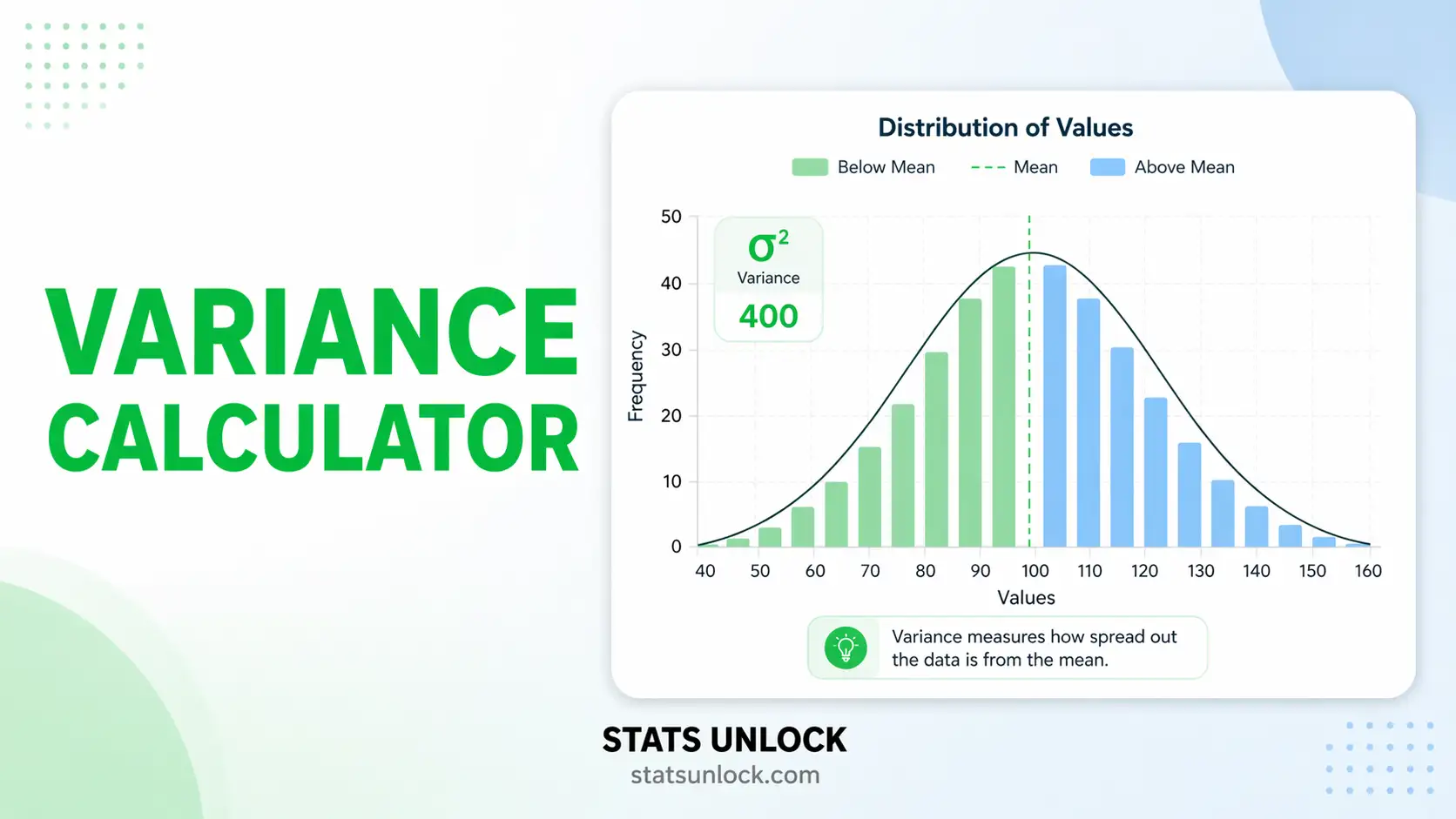
Variance measures how far data values are spread from their mean. It is the average of the squared deviations from the mean. You should use a variance calculator anytime you need to quantify data dispersion — for example, comparing the consistency of exam scores, the variability in animal body weights, or the spread in manufacturing tolerances. Our online variance calculator handles both population and sample variance in seconds.

Population variance (σ²) is calculated by dividing the sum of squared deviations by N (the total number of data points). Sample variance (s²) divides by n−1 instead of n. This one-less correction — called Bessel's correction — compensates for the fact that a sample mean is closer to the sample values than the true population mean is, which causes raw sample deviations to underestimate the true spread. Use population variance only when you have measured every member of the group.

Bessel's correction is the use of n−1 (instead of n) in the denominator when computing sample variance. It was derived by Friedrich Bessel to produce an unbiased estimator of the population variance. Without it, sample variance consistently underestimates the true spread of the population. For large samples (n > 30) the difference is small; for small samples it can be substantial.

High variance means values are spread far from the mean — the data is inconsistent or heterogeneous. Low variance means values cluster tightly around the mean — the data is consistent or homogeneous. The interpretation is always context-dependent: a variance of 4 is tiny for body weight in kilograms but enormous for room temperature in degrees Celsius. Always compare variance in the same units and on similar scales.

Standard deviation is simply the square root of variance: SD = √Variance. Variance is expressed in squared units (e.g., kg², cm²) which are hard to interpret intuitively. Standard deviation brings the spread back to the original units, making it easier to communicate. Both are used frequently in research; variance is mathematically central (it's what ANOVA partitions), while SD is preferred for descriptive reporting.

No — variance can never be negative. Because each deviation is squared before summing, the result is always ≥ 0. The only way variance equals zero is if every value in the dataset is identical (no spread at all). If you see a negative variance result somewhere, it indicates a calculation error.

For APA-style papers and most journals, report the Standard Deviation (SD) alongside the mean because it is in the same units as your measurement. Report variance when the analysis itself involves variance directly — for example, when discussing ANOVA results, effect sizes (η²), or comparing measurement instrument reliability. Always follow the journal's style guide; many now require effect sizes and CIs alongside SD.

Variance is in squared units of the original measurement. If your data is in metres, variance is in m². If your data is in kilograms, variance is in kg². This squared nature makes variance difficult to interpret directly. To get back to the original units, take the square root (standard deviation). Alternatively, use the Coefficient of Variation (CV = SD/Mean × 100%) to express relative variability as a percentage — this is unit-free and useful for comparing datasets measured on different scales.

The coefficient of variation (CV) = (Standard Deviation / Mean) × 100%. It normalises variability relative to the mean, allowing comparison across datasets with different units or scales. For example, comparing the CV of bird wing lengths (cm) with fish body weights (g) is meaningful, whereas comparing their raw variances is not. A CV below 15% is often considered low variability; above 30% indicates high variability.

A minimum of 30 observations is the general rule of thumb for variance estimates to be stable and reasonably close to the true population variance. With very small samples (n < 10), variance estimates are highly sensitive to individual values and can change dramatically if one value changes. For skewed or heavy-tailed data, 50+ observations produce more reliable estimates. Our calculator computes variance for any n ≥ 2, but always consider sample size when interpreting results.