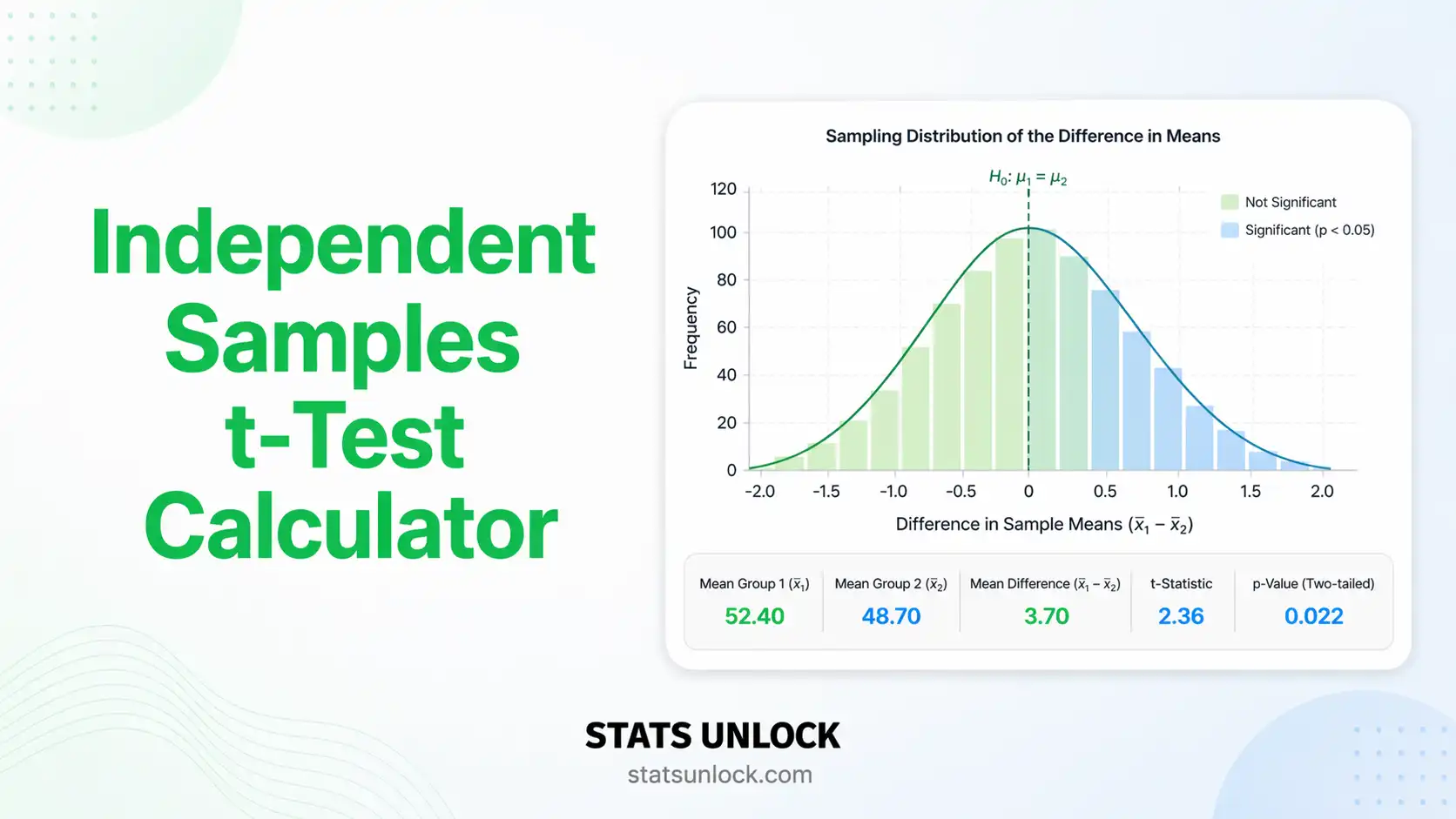
Independent Samples t-Test Calculator
Compare two independent group means with instant t-statistic, p-value, degrees of freedom, Cohen's d effect size, 95% confidence interval, and APA-ready results. Free, no software required.
| Group 1 | Group 2 |
|---|
Formulas Used
Technical Notes
- Welch's correction (default): Does not assume equal variances; uses Satterthwaite approximation for degrees of freedom. Recommended for most real-world data.
- Student's t-test: Assumes equal population variances. More powerful than Welch's when assumption holds; less robust when it doesn't.
- p-value computed from t-distribution CDF with the calculated degrees of freedom.
- Cohen's d benchmarks: Small ≈ 0.2, Medium ≈ 0.5, Large ≈ 0.8 (Cohen, 1988).
- Normality: Central Limit Theorem applies for n ≥ 30 per group. For smaller samples, verify with Shapiro-Wilk or Q-Q plots.
- Independence: Each observation must belong to exactly one group. If the same participants are measured twice, use the Paired t-test.
The independent samples t-test answers one question: Do two separate, unrelated groups have different population means? It is the most commonly used parametric test for comparing two groups on a continuous outcome.
Decision Checklist
- ✅ You have exactly two independent groups (participants in one group cannot be in the other)
- ✅ Your dependent variable is continuous (interval or ratio scale — e.g., weight, score, time)
- ✅ Data within each group are approximately normally distributed, OR n > 30 per group (CLT applies)
- ✅ Observations are independent — no repeated measurements, no matching
- ❌ Do NOT use if groups are paired or matched → use Paired t-test
- ❌ Do NOT use if you have 3+ groups → use One-Way ANOVA
- ❌ Do NOT use if data are ordinal or heavily skewed with small n → use Mann-Whitney U
Real-World Examples
Comparing mean systolic blood pressure between a drug-treatment group and a placebo group after a 4-week trial to determine if the drug significantly reduces blood pressure.
Comparing final exam scores between students taught with a flipped classroom method versus a traditional lecture method to assess which approach is more effective.
Comparing self-reported anxiety scores (GAD-7) between two demographic groups (e.g., urban vs rural residents) to examine the effect of living environment on mental health.
Comparing average purchase values between customers who received a promotional email and those who did not, to quantify the campaign's effect on revenue.
Related Tests — Decision Tree
Sample Size Guidance
Minimum: 15–20 per group for normal data. For 80% power to detect a medium effect (d = 0.5, α = 0.05), approximately 64 participants total (32 per group) are needed. Fewer than 10 per group makes results unreliable regardless of p-value.
52, 48, 55, 61, 47). Edit the group name above the textarea.What is the independent samples t-test and when should I use it?
The independent samples t-test (also called the two-sample t-test) compares the means of two separate, unrelated groups to determine whether they differ significantly. Use it when you have one continuous dependent variable measured in two non-overlapping groups — for example, comparing exam scores between a control class and an experimental class, or blood pressure between a drug and placebo group.
What is a p-value and how do I interpret it for this test?
The p-value is the probability of observing a difference as large as (or larger than) yours, if the null hypothesis (no real difference between groups) were true. A p-value of 0.03 means there is a 3% chance of seeing this result by chance alone. It does NOT mean there is a 3% chance the null hypothesis is true — that is a common misconception.
Convention: p < 0.05 is considered statistically significant, though this threshold is arbitrary. Always report the exact p-value, not just "significant" or "not significant."
What does statistical significance mean — and does it equal practical importance?
Statistical significance (p < α) tells you only that the result is unlikely to be due to chance. It does not tell you the effect is large, meaningful, or clinically important. With very large samples, trivially small differences can produce p < 0.001. This is why effect size (Cohen's d) is equally important — it quantifies the magnitude, not just the presence, of a difference.
What is Cohen's d and how do I interpret it?
Cohen's d is the standardised mean difference — it tells you how many standard deviations apart the two group means are. Benchmarks from Cohen (1988): d = 0.2 = small, d = 0.5 = medium, d = 0.8 = large. A d of 0.8 means the groups differ by 0.8 standard deviations — a difference that would be clearly visible in a side-by-side distribution plot.
Cohen's d does not depend on sample size, making it useful for comparing findings across studies.
What assumptions does the independent samples t-test require, and what if they're violated?
1. Independence: Observations in one group must not influence the other group. If the same participants are measured twice, use the Paired t-test instead.
2. Continuous DV: The dependent variable must be on an interval or ratio scale.
3. Normality: Data within each group should be approximately normal. For n > 30 per group, the Central Limit Theorem makes the test robust. For smaller samples, check with Q-Q plots or Shapiro-Wilk. If violated: use the Mann-Whitney U test.
4. Homogeneity of variances: Use Welch's correction (selected by default here) when variances may differ — it is robust whether or not variances are equal.
How large a sample do I need for the test to be reliable?
Rule of thumb: at least 15–20 participants per group for approximately normal data. For 80% statistical power to detect a medium effect (d = 0.5) at α = 0.05, you need approximately 64 total (32 per group). For a small effect (d = 0.2), you need approximately 394 total. Fewer than 10 per group makes results unreliable even if p < 0.05. When sample sizes are very small, consider non-parametric alternatives.
What is the difference between one-tailed and two-tailed testing, and which should I choose?
A two-tailed test tests whether the means differ in either direction (Group 1 > Group 2 or Group 1 < Group 2). A one-tailed test tests only one direction and is more powerful — but requires the directional hypothesis to be stated before data collection.
General recommendation: always use two-tailed tests unless you have a strong, pre-specified theoretical reason to expect the effect in one direction only. Switching to one-tailed after seeing data (to achieve significance) is a serious statistical error.
How do I report independent samples t-test results in APA 7th edition format?
APA format: "An independent-samples t-test was conducted to compare [DV] between [Group 1] and [Group 2]. Results indicated a [significant/non-significant] difference between [Group 1] (M = ___, SD = ___) and [Group 2] (M = ___, SD = ___), t(___) = ___, p [
Rules: italicise all statistical symbols (t, p, M, SD, d); report p to three decimal places; write "p < .001" not "p = .000"; always include effect size.
Run the analysis above to get five auto-filled reporting templates including APA, Thesis, Plain-Language, Abstract, and Pre-Registration styles.
Can I use this calculator for published research or a university assignment?
This tool is designed for educational use and exploratory analysis. Results are mathematically accurate for clean, well-entered data. For formal research submissions, verify results with peer-reviewed statistical software such as R (t.test()), Python (scipy.stats.ttest_ind), SPSS, or SAS. To cite this tool: STATS UNLOCK. (2025). Independent samples t-test calculator. Retrieved from https://statsunlock.com/independent-samples-t-test-calculator
What should I do if my results are non-significant — does that mean my hypothesis is wrong?
A non-significant result (p > α) does not prove the null hypothesis is true. It only means the current data do not provide sufficient evidence to reject it. Possible reasons: insufficient sample size (Type II error), a genuinely small or absent effect, or high variability in the data.
Next steps: check whether your study had enough statistical power to detect your expected effect size; consider a larger replication; or use a Bayes Factor analysis to quantify evidence for the null hypothesis rather than simply failing to reject it.
Use this calculator to determine the minimum sample size needed per group before you collect data, or to check the statistical power of an already-completed study. Enter any three values to compute the fourth.
Cohen's d Effect Size Reference
| Label | Cohen's d | Meaning | n per group (α=.05, power=80%) |
|---|---|---|---|
| Negligible | < 0.2 | Difference barely detectable; likely not practically meaningful | > 394 |
| Small | 0.2 | Subtle effect — visible only in large samples or sensitive measures | 394 |
| Medium | 0.5 | Moderate effect — noticeable to a careful observer | 64 |
| Large | 0.8 | Obvious effect — clearly visible without statistics | 26 |
| Very Large | ≥ 1.2 | Dramatic effect — groups barely overlap in distribution | 12 |
How to Read This
- Power (1 − β): The probability of correctly detecting a real effect. 0.80 (80%) is the conventional minimum — it means a 20% risk of a false negative (missing a real effect).
- Type I error (α): The probability of a false positive — detecting an effect that doesn't exist. Conventionally set at 0.05.
- Underpowered studies (power < 0.80) frequently produce non-significant results even when a real effect exists. Always plan sample size before data collection.
- Achieved power: If you've already collected data, enter your actual n per group to see how much power your study had.
The following references support the statistical methods used in this calculator, covering effect size interpretation, p-value reporting, and best practices in hypothesis testing and parametric statistical analysis.
- Student [Gosset, W. S.]. (1908). The probable error of a mean. Biometrika, 6(1), 1–25. https://doi.org/10.1093/biomet/6.1.1
- Welch, B. L. (1947). The generalization of "Student's" problem when several different population variances are involved. Biometrika, 34(1–2), 28–35. https://doi.org/10.1093/biomet/34.1-2.28
- Cohen, J. (1988). Statistical power analysis for the behavioral sciences (2nd ed.). Lawrence Erlbaum Associates.
- American Psychological Association. (2020). Publication manual of the American Psychological Association (7th ed.). https://doi.org/10.1037/0000165-000
- Field, A. (2018). Discovering statistics using IBM SPSS statistics (5th ed.). SAGE Publications.
- Gravetter, F. J., & Wallnau, L. B. (2021). Statistics for the behavioral sciences (10th ed.). Cengage Learning.
- Cumming, G. (2014). The new statistics: Why and how. Psychological Science, 25(1), 7–29. https://doi.org/10.1177/0956797613504966
- Lakens, D. (2013). Calculating and reporting effect sizes to facilitate cumulative science: A practical primer for t-tests and ANOVAs. Frontiers in Psychology, 4, 863. https://doi.org/10.3389/fpsyg.2013.00863
- Sullivan, G. M., & Feinn, R. (2012). Using effect size — or why the P value is not enough. Journal of Graduate Medical Education, 4(3), 279–282. https://doi.org/10.4300/JGME-D-12-00156.1
- Ruxton, G. D. (2006). The unequal variance t-test is an underused alternative to Student's t-test and the Mann-Whitney U test. Behavioral Ecology, 17(4), 688–690. https://doi.org/10.1093/beheco/ark016
- Wasserstein, R. L., & Lazar, N. A. (2016). The ASA statement on p-values: Context, process, and purpose. The American Statistician, 70(2), 129–133. https://doi.org/10.1080/00031305.2016.1154108
- R Core Team. (2024). R: A language and environment for statistical computing. R Foundation for Statistical Computing. https://www.R-project.org/
- Virtanen, P., et al. (2020). SciPy 1.0: Fundamental algorithms for scientific computing in Python. Nature Methods, 17, 261–272. https://doi.org/10.1038/s41592-019-0686-2
- NIST/SEMATECH. (2013). e-Handbook of statistical methods. https://www.itl.nist.gov/div898/handbook/


