

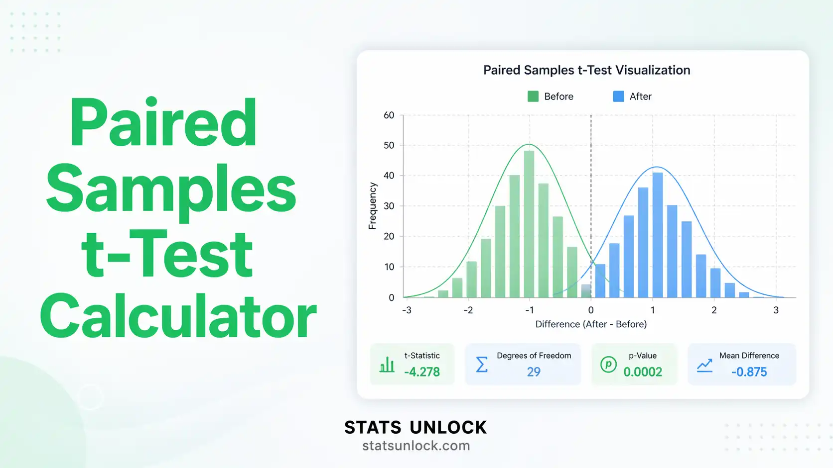

Paired Samples t-Test Calculator
Compare two related measurements from the same subjects — pre/post tests, matched pairs, repeated measures. Get instant results with full APA reporting, Cohen's d effect size, and detailed interpretation.
Enter values comma-separated or one per line. Both groups must have the same number of values. Decimal values (e.g. 3.14) are supported.
Headers are detected automatically. Supports .csv, .txt, .xlsx, .xls — click on column buttons to assign each column as a group. Selected columns load as separate paired groups.
Enter paired values directly in the table below. Each row = one pair of observations.
| Pair # | Pre-Test | Post-Test |
|---|
🔍 Assumption Checks ▼
💬 Interpretation of Results ▼
✍️ How to Write Your Results in Research ▼
🔢 Technical Notes & Formulas ▼
Formulas Used
Technical Notes
The paired t-test is mathematically equivalent to a one-sample t-test applied to the differences. By explicitly modelling within-subject pairing, it eliminates between-subject variance, producing a smaller standard error and higher statistical power than an independent t-test on the same data, provided the correlation between paired measurements is positive and substantial (r > 0.3).
If normality of differences is violated (Shapiro-Wilk p < .05) and n < 30, consider the Wilcoxon Signed-Rank Test as a non-parametric alternative. For samples with n > 30, the Central Limit Theorem ensures the t-statistic remains approximately normally distributed even with moderate non-normality.
The two-tailed p-value is computed as: p = 2 × P(T > |t|) where T ~ t(n−1). One-tailed p-values use the appropriate tail only.
🎯 When to Use the Paired Samples t-Test ▼
The paired samples t-test is the right choice when you have two measurements that are logically linked — either because the same subject was measured twice, or because two subjects were deliberately matched before measurement.
Decision Checklist
Real-World Examples
🩺 Medicine — Pre/Post Drug Trial
A cardiologist measures systolic blood pressure in 20 patients before and after 8 weeks of a new antihypertensive drug. Each patient is their own control. The paired t-test removes the huge between-patient variability in baseline blood pressure, revealing whether the drug itself caused a change.
🎓 Education — Tutoring Effectiveness
A school measures mathematics test scores for 30 students before and after a one-month tutoring programme. The paired t-test tests whether scores improved on average, controlling for each student's initial ability level.
🧠 Psychology — Cognitive Training
Researchers measure reaction time in 25 participants before and after a 6-week cognitive training intervention. The paired design ensures that slower participants don't simply inflate the pre-training group mean.
🌿 Ecology — Habitat Paired Comparison
A wildlife biologist measures species richness in 18 forest plots before and after a selective logging operation. Plots are naturally matched by location, so the paired test captures the within-plot change, not between-plot variation in baseline richness.
Related Tests — Decision Tree
Sample Size & Power
- For 80% power, medium effect (d=0.5), α=.05 two-tailed: ~34 pairs needed
- For 80% power, small effect (d=0.2), α=.05 two-tailed: ~198 pairs needed
- For 80% power, large effect (d=0.8), α=.05 two-tailed: ~15 pairs needed
- Minimum for reliable inference: ≥ 10 pairs (normality very hard to verify below this)
- Higher correlation between repeated measures = more power (more reason to use paired design)
📖 How to Use This Calculator — Step-by-Step Guide ▼
Enter Your Data
Choose one of three input methods: type/paste values directly into the text boxes (comma-separated or one per line), upload a CSV or Excel file and click the columns you want to assign, or use the manual entry grid. Both groups must have the same number of values (one per pair). Example: Pre-Test: 52, 48, 55, 61, 47 | Post-Test: 48, 44, 50, 55, 43
Name Your Groups (Optional)
Edit the "Group 1 Name" and "Group 2 Name" fields to match your study design — these names appear in all results and reports. Examples: "Before Training / After Training", "Control / Treatment", "Time 1 / Time 2".
Choose a Sample Dataset
Not sure what your data should look like? Select one of 5 built-in datasets from the dropdown to see how the tool works. Options include blood pressure treatment, exam score tutoring, running speed training, stress interventions, and a crossover drug trial. Click "Run Paired t-Test" to see full results.
Configure Test Settings
Choose your significance level (α = 0.01, 0.05, or 0.10), and tail type (two-tailed recommended unless you have a pre-specified directional hypothesis). The confidence level automatically updates to match your α choice.
Run the Analysis
Click the green "Run Paired t-Test" button. Results appear instantly — no page reload. Example output: t(11) = 3.42, p = .005, d = 0.89
Read the Summary Cards
The four coloured cards at the top show your key values at a glance. Green = significant, amber = borderline, red = not significant. Each card shows the statistic name and value.
Examine the Four Visualizations
(1) Differences histogram: shows if the differences are approximately normal. (2) t-distribution curve: shows where your t-statistic falls relative to critical values. (3) Box plot: compares the two groups side by side. (4) Spaghetti plot: shows each subject's individual change from Time 1 to Time 2.
Check the Assumption Verification Panel
Green badges = assumption met. Amber = borderline, proceed with caution. Red = assumption violated. If normality fails and n < 30, consider using the Wilcoxon Signed-Rank Test instead.
Read the Detailed Interpretation
The interpretation section explains your results in plain English, covering what the p-value means, what the effect size means in practical terms, limitations, and whether the result is practically important (not just statistically significant).
Copy a Reporting Template & Export
Choose one of 5 auto-filled reporting templates (APA 7th, Thesis, Plain Language, Abstract, Pre-Registration) and click "Copy" to paste directly into your paper. Download a full report as a .txt Doc or a print-ready PDF.
❓ Frequently Asked Questions ▼
Q1. What is the paired samples t-test and when should I use it?
The paired samples t-test (also called the dependent samples t-test, repeated measures t-test, or matched pairs t-test) compares the means of two related measurements. Use it when the same subjects are measured twice — for example, before and after an intervention — or when two subjects are deliberately matched on important characteristics. By computing the difference for each pair, the test removes between-subject variability, making it more statistically powerful than an independent t-test for matched designs.
Common applications include pre-test/post-test educational studies, crossover clinical trials, left-eye vs right-eye medical measurements, and paired ecological transects.
Q2. What is a p-value, and how do I interpret it in the paired t-test?
The p-value is the probability of observing a mean difference as large as yours (or larger) if there were truly no difference between the two conditions — in other words, if chance alone were operating. A p-value of 0.03 means there is a 3% chance of seeing a difference this large by chance.
Important: the p-value is NOT the probability that the null hypothesis is true, and it is NOT the probability of making an error. A p-value below your chosen α (e.g., .05) means you reject the null hypothesis — but always look at the effect size to judge whether the difference is practically meaningful.
Q3. What does statistical significance mean — and does it equal practical importance?
Statistical significance (p < α) tells you that the observed difference is unlikely to be due to chance at your chosen threshold. It does NOT tell you whether the difference is large enough to matter in practice.
With a very large sample (e.g., n = 5,000 pairs), even a trivially small mean difference (e.g., 0.1 mmHg blood pressure change) will be statistically significant. That's why you must always report and interpret the effect size (Cohen's d) alongside the p-value. A difference can be statistically significant but practically negligible — or practically important even when p is slightly above .05 (consider the power of your study).
Q4. What is Cohen's d and how do I interpret it for a paired t-test?
Cohen's d for the paired t-test is calculated as the mean difference divided by the standard deviation of the differences (d̄ / s_d). It tells you how large the mean change is relative to the variability in change scores.
Cohen's (1988) benchmarks: d = 0.2 = small (small but real effect, roughly the difference between heights of 15- and 16-year-old girls); d = 0.5 = medium (noticeable to careful observers, e.g. a moderate intervention effect); d = 0.8 = large (obvious to any observer, e.g. a highly effective treatment). Note that these benchmarks were designed for social sciences — in medical research, a d of 0.2 may still be clinically meaningful if the outcome is mortality.
Q5. What assumptions does the paired t-test require, and what if they're violated?
The paired t-test requires: (1) Paired / related observations — each value in Group 1 must correspond to one specific value in Group 2; (2) Normality of differences — the d_i = x1_i − x2_i values should be approximately normally distributed (verified by Shapiro-Wilk test or Q-Q plot); (3) No extreme outliers in the differences — a single outlier can dramatically inflate the SD and distort the result; (4) Continuous or interval measurement — the test is not valid for ordinal or nominal data.
If normality is violated and n < 30: use the Wilcoxon Signed-Rank Test. If you have only ordinal data: use Wilcoxon Signed-Rank Test. If n > 30: the Central Limit Theorem means non-normality is less critical, and you can usually proceed.
Q6. How many pairs do I need for the paired t-test to be reliable?
The minimum number of pairs depends on the size of the effect you want to detect. For 80% power at α = .05 (two-tailed): detecting a large effect (d = 0.8) requires approximately 15 pairs; detecting a medium effect (d = 0.5) requires approximately 34 pairs; detecting a small effect (d = 0.2) requires approximately 198 pairs.
With fewer than 10 pairs, the normality assumption becomes almost impossible to verify, and the test can be unreliable even if p < .05. Samples with 5–9 pairs should be treated with caution and supplemented with a Wilcoxon Signed-Rank test for verification.
Q7. What is the difference between a one-tailed and two-tailed paired t-test?
A two-tailed test detects a mean difference in either direction (Group 1 could be higher OR lower than Group 2). A one-tailed test tests only one direction — either that Group 1 is higher (right-tailed) or that Group 1 is lower (left-tailed). One-tailed tests are more powerful (easier to reach significance) but must be justified by a strong, pre-specified directional hypothesis made before data collection.
Recommendation: use a two-tailed test by default. Applying a one-tailed test after seeing your data direction is considered p-hacking and can inflate the Type I error rate. Only switch to one-tailed if your pre-registration or study protocol explicitly committed to a directional hypothesis.
Q8. How do I report paired t-test results in APA 7th edition format?
APA 7th edition requires the test name, means and SDs of both groups, the t-statistic, degrees of freedom, exact p-value (or "p < .001"), effect size (Cohen's d), and confidence interval.
Example: "A paired samples t-test was conducted to assess whether blood pressure changed from pre-treatment (M = 148.3, SD = 9.2) to post-treatment (M = 135.7, SD = 8.6). Results indicated a statistically significant decrease, t(11) = 4.23, p = .001, d = 1.22, 95% CI [6.1, 19.2] mmHg." Note: use italics for all statistical symbols in actual manuscripts. See the "How to Write Your Results" section above for all 5 reporting templates.
Q9. Can I use this calculator for published research or university assignments?
This calculator is designed for education, learning, and exploratory data analysis. The computational formulas used are standard and accurate. For formal publication, always verify results using peer-reviewed statistical software such as R (base::t.test), Python (scipy.stats.ttest_rel), SPSS, SAS, or Stata.
To cite this tool in your work: StatsUnlock. (2025). Paired samples t-test calculator. Retrieved from https://statsunlock.com/tools/paired-samples-t-test-calculator/
Q10. My result is non-significant — does that mean there's no effect?
No. A non-significant result (p > α) does not prove there is no effect — it means your data do not provide sufficient evidence to reject the null hypothesis at your chosen significance level. This could be because: (a) there genuinely is no meaningful effect, (b) your sample size was too small to detect the effect (low statistical power), or (c) the effect size is smaller than your study was designed to detect.
Always check the confidence interval for the mean difference. If the entire CI is within your "practically unimportant" zone, you can more confidently conclude the effect is negligible. If the CI is wide or overlaps meaningful values, the result is inconclusive — not negative. Consider a Bayesian analysis (Bayes Factor) to quantify evidence in favor of the null hypothesis.
📚 References ▼
The following peer-reviewed references support the statistical methods, paired samples t-test formulas, effect size interpretation, and reporting guidelines used in this paired t-test calculator and paired difference t-test tool.
- Student [W. S. Gosset]. (1908). The probable error of a mean. Biometrika, 6(1), 1–25. https://doi.org/10.1093/biomet/6.1.1
- Cohen, J. (1988). Statistical power analysis for the behavioral sciences (2nd ed.). Lawrence Erlbaum Associates.
- Lakens, D. (2013). Calculating and reporting effect sizes to facilitate cumulative science: A practical primer for t-tests and ANOVAs. Frontiers in Psychology, 4, 863. https://doi.org/10.3389/fpsyg.2013.00863
- Cumming, G. (2014). The new statistics: Why and how. Psychological Science, 25(1), 7–29. https://doi.org/10.1177/0956797613504966
- Sullivan, G. M., & Feinn, R. (2012). Using effect size — or why the p value is not enough. Journal of Graduate Medical Education, 4(3), 279–282. https://doi.org/10.4300/JGME-D-12-00156.1
- Wilcoxon, F. (1945). Individual comparisons by ranking methods. Biometrics Bulletin, 1(6), 80–83. https://doi.org/10.2307/3001968
- Royston, P. (1995). Remark AS R94: A remark on Algorithm AS 181: The W test for normality. Journal of the Royal Statistical Society: Series C, 44(4), 547–551. https://doi.org/10.2307/2986146
- American Psychological Association. (2020). Publication manual of the American Psychological Association (7th ed.). APA. https://doi.org/10.1037/0000165-000
- Wasserstein, R. L., & Lazar, N. A. (2016). The ASA's statement on p-values: Context, process, and purpose. The American Statistician, 70(2), 129–133. https://doi.org/10.1080/00031305.2016.1154108
- Kelley, K., & Preacher, K. J. (2012). On effect size. Psychological Methods, 17(2), 137–152. https://doi.org/10.1037/a0028086
- Faul, F., Erdfelder, E., Lang, A.-G., & Buchner, A. (2007). G*Power 3: A flexible statistical power analysis program for the social, behavioral, and biomedical sciences. Behavior Research Methods, 39(2), 175–191. https://doi.org/10.3758/BF03193146
- Field, A. (2018). Discovering statistics using IBM SPSS Statistics (5th ed.). SAGE Publications. https://doi.org/10.4135/9781526419521
- Grissom, R. J., & Kim, J. J. (2005). Effect sizes for research: A broad practical approach. Lawrence Erlbaum Associates. https://doi.org/10.4324/9781410612915
- Virtanen, P., Gommers, R., Oliphant, T. E., et al. (2020). SciPy 1.0: Fundamental algorithms for scientific computing in Python. Nature Methods, 17, 261–272. https://doi.org/10.1038/s41592-020-0772-5
- R Core Team. (2024). R: A language and environment for statistical computing. R Foundation for Statistical Computing. https://www.R-project.org/