📈 SARIMA Model Calculator
Free online Seasonal ARIMA (SARIMA) tool — enter your time series data, set model parameters, and get instant forecasts, ACF/PACF diagnostics, AIC/BIC model selection, and publication-ready write-ups.
📥 Enter Your Time Series Data
Click to browse or drag & drop your file here
Accepts .csv, .txt, .xlsx, .xls — click column buttons to select your time series
| Time Index | Value |
|---|
⚙️ SARIMA Model Configuration
🧮 Technical Notes — SARIMA Formulas & Definitions
The SARIMA model combines non-seasonal and seasonal ARIMA components. Below are the core formulas used in this calculator.
🧭 When to Use SARIMA — Decision Guide
This free SARIMA model calculator is designed for researchers, analysts, and students who need to forecast time series data with regular seasonal patterns. SARIMA is ideal when your series shows both non-stationarity (trend) and periodic seasonality.
✅ Use SARIMA when:
- ✓ Your data has a clear repeating seasonal cycle (e.g., annual, quarterly, monthly)
- ✓ The series is non-stationary (mean or variance changes over time)
- ✓ You have at least 3–4 full seasonal cycles of observations (e.g., 36+ months for s=12)
- ✓ The ACF shows significant spikes at multiples of the seasonal period
- ✓ You want to produce short- to medium-horizon forecasts with confidence intervals
- ✗ Do NOT use if data has no seasonal pattern → use ARIMA instead
- ✗ Do NOT use if seasonality changes in amplitude over time → consider ETS multiplicative or STL decomposition first
- ✗ Do NOT use if you have fewer than 2 seasonal cycles of data → insufficient for reliable estimation
- ✗ Do NOT use if the series contains many missing values → handle gaps before fitting
🌍 Real-World Examples
📦 Retail & Supply Chain
Monthly retail sales showing holiday peaks in November–December. SARIMA(1,1,1)(1,1,1)[12] captures both year-over-year growth and seasonal spikes to forecast inventory needs.
🌡️ Climate & Environment
Monthly average temperatures with clear annual cycles. Wildlife biologists use SARIMA to forecast seasonal animal activity periods, migration timing, or rainfall-dependent resource availability.
📈 Economics & Finance
Quarterly GDP growth with recurring seasonal dips in Q1. Economists fit SARIMA models to produce business cycle forecasts and inform policy decisions with uncertainty bands.
🏥 Public Health
Weekly influenza cases with annual winter peaks. Epidemiologists use SARIMA to anticipate hospital demand surges and allocate resources weeks in advance.
🌳 Model Selection Decision Tree
📖 How to Use This SARIMA Calculator — Step-by-Step Guide
Follow these 10 steps to run a complete SARIMA analysis using this free time series forecasting tool.
Type or paste your time series values in the input box (comma-separated: e.g.,
52, 48, 55, 61, 47, ...), upload a CSV/Excel file and select your column, or use the manual grid. Edit the Series Name field to label your data. You need at least 24 observations; 48+ is recommended for seasonal models.If you want to explore the tool first, select one of 5 built-in datasets from the dropdown and click "Load Sample". Sample 1 (Monthly Retail Sales) is pre-loaded. Each sample covers a different domain and seasonal period.
Set p, d, q (non-seasonal) and P, D, Q, s (seasonal). A good starting point for monthly data with trend and seasonality is SARIMA(1,1,1)(1,1,1)[12]. For quarterly data, try (1,1,1)(1,1,1)[4]. If unsure, start with d=1, D=1, and examine ACF/PACF plots after the first run to refine p, q, P, Q.
Choose how many steps ahead to forecast (6, 12, 24, or 36 steps). Select your confidence level for forecast intervals (95% is standard in research). Set your significance level α (0.05 is the default).
Click "▶ Run SARIMA Analysis". Results appear immediately. The calculator fits the model, computes fitted values, generates forecasts, calculates AIC/BIC, and runs Ljung-Box residual diagnostics.
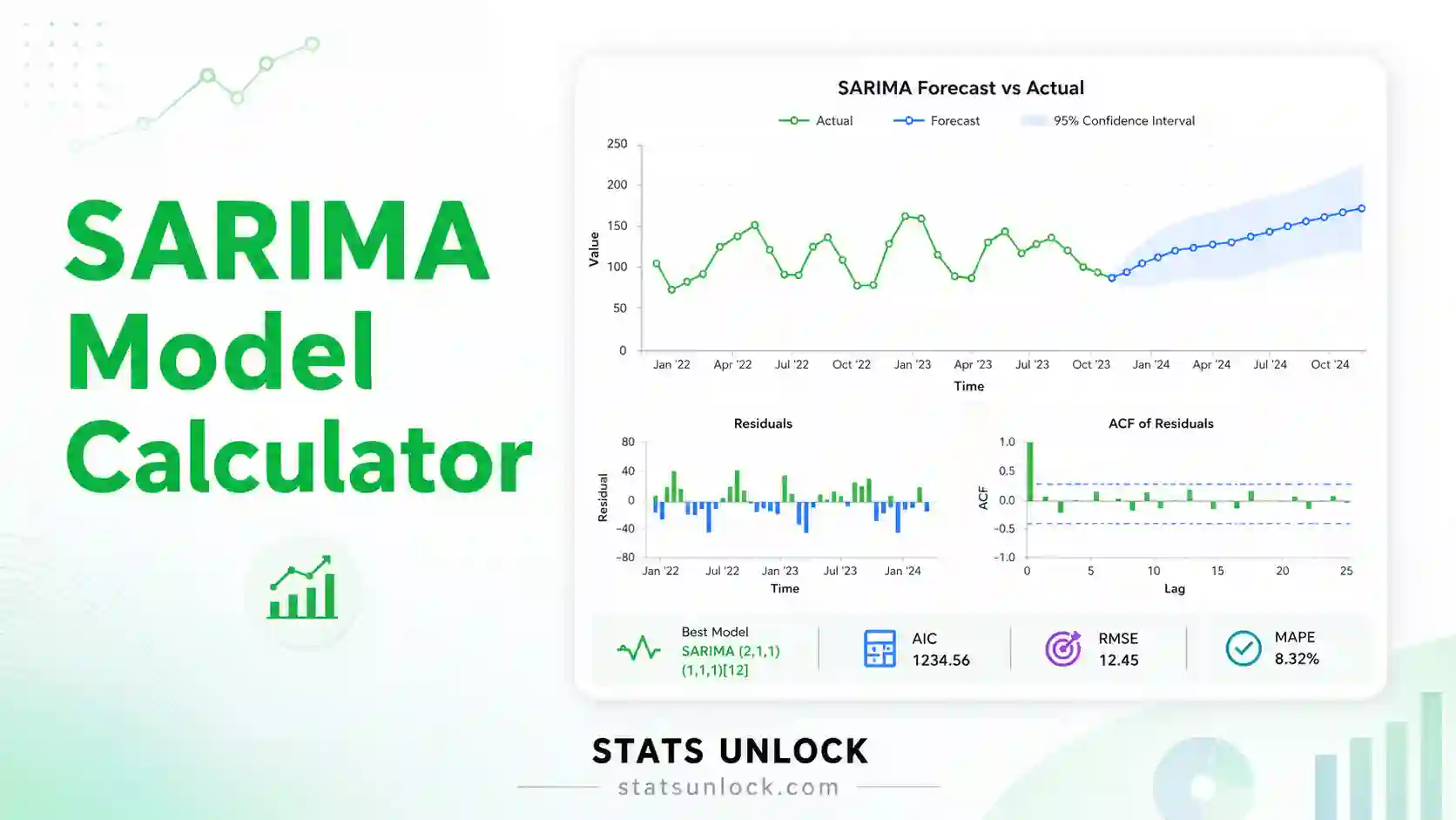
Six coloured stat cards show: Model specification (e.g., SARIMA(1,1,1)(1,1,1)[12]), AIC, BIC, RMSE, MAPE, and Ljung-Box p-value. AIC/BIC lower = better fit. MAPE below 10% = excellent forecast accuracy. Ljung-Box p > 0.05 = residuals are white noise (good).
① Original series + fitted values: fitted line should track the data well. ② Forecast plot: shaded region = confidence interval — should widen into the future. ③ ACF of residuals: bars should stay within the blue confidence bands (no significant autocorrelation). ④ Residuals over time: should look like random noise with no pattern.
The Diagnostic Checks panel shows green ✓ (pass), orange ⚠ (warning), or red ✗ (fail) badges for: data length, stationarity after differencing, Ljung-Box test, normality of residuals, and residual mean. Fix failures by adjusting parameters — if Ljung-Box fails, try increasing q or Q.
The Interpretation Results section gives 5 detailed paragraphs explaining your SARIMA model results in plain English. Below that, five write-up templates are auto-filled with your actual computed values — copy any template for your APA journal article, thesis, policy report, conference abstract, or pre-registration.
Click "Download Report (.txt)" for a plain-text file with all results (ideal for supplementary materials). Click "Save as PDF" to print a formatted A4 report — select "Save as PDF" in your browser's print dialog. Both exports include the full analysis, interpretation, and write-up templates.
❓ Frequently Asked Questions — SARIMA Model
Q1. What is a SARIMA model and when should I use it?
SARIMA stands for Seasonal AutoRegressive Integrated Moving Average. It extends the standard ARIMA model by adding seasonal AR, differencing, and MA components that operate at seasonal lags. Use SARIMA when your time series data shows a repeating seasonal pattern over a fixed period — such as monthly sales data that peaks every holiday season, quarterly GDP that dips every Q1, or weekly website traffic that spikes every Monday. The model is written as SARIMA(p,d,q)(P,D,Q)[s], where s is the seasonal period.
Q2. What do the SARIMA parameters p, d, q, P, D, Q, and s mean?
Each parameter controls a specific part of the model: p = number of past values (lags) used in the non-seasonal autoregressive component; d = number of times the series is differenced to remove a trend; q = number of past forecast errors in the non-seasonal moving average; P = seasonal AR order (how many seasonal lags); D = seasonal differencing (removes seasonal trend); Q = seasonal MA order; s = number of time steps per season (12 for monthly, 4 for quarterly, 7 for daily-within-weekly). Choosing appropriate values requires inspecting ACF and PACF plots and comparing AIC/BIC across candidate models.
Q3. How do I choose the right values for p, d, q, P, D, Q?
Start by plotting the series and checking for trend (d) and seasonal non-stationarity (D). If the series drifts upward, set d=1. If the seasonal amplitude changes year over year, set D=1. After differencing, inspect the ACF: significant spikes at lag 1, 2, … suggest q; spikes at lag s, 2s, … suggest Q. Inspect the PACF: spikes at lag 1, 2, … suggest p; spikes at lag s, 2s, … suggest P. Fit several candidate models and compare their AIC and BIC — lower values indicate a better fit. Always verify with the Ljung-Box test on residuals: a non-significant result (p > 0.05) means the model has captured all autocorrelation.
Q4. What is AIC and BIC, and which should I minimise?
AIC (Akaike Information Criterion) and BIC (Bayesian Information Criterion) both balance model fit (log-likelihood) against model complexity (number of parameters). Lower values are better — they indicate a model that fits the data well without overfitting. BIC applies a stronger penalty for additional parameters, so it tends to select simpler models than AIC. In practice, if AIC and BIC disagree, prefer BIC for parsimony in short series (n < 100) and AIC for predictive accuracy in longer series. Differences of less than 2 units between models are not meaningful.
Q5. What does the Ljung-Box test tell me about my SARIMA model?
The Ljung-Box test checks whether the residuals from your fitted SARIMA model are uncorrelated (white noise). The null hypothesis is that all autocorrelations in the residuals up to lag h are zero. A non-significant result (p > 0.05) means the model has successfully removed all autocorrelation from the data — this is what you want. A significant result (p ≤ 0.05) means residual autocorrelation remains, and the model is inadequate. Try increasing q or Q, or adding one more AR term. Always test at lag h = min(2s, n/5) for seasonal models.
Q6. How do I interpret the SARIMA forecast and its confidence intervals?
The point forecast is the model's single best estimate of each future value, generated by propagating the fitted model equations forward. The confidence interval (CI) is the range in which the true future value is expected to fall with the stated probability (e.g., 95%). The CI widens with the forecast horizon because uncertainty accumulates. A 95% CI means that if you repeated this process many times, 95% of the intervals would contain the true value. In practice, SARIMA forecasts are most reliable within 1–2 seasonal cycles; beyond that, uncertainty can be very large.
Q7. What is MAPE and how do I judge forecast accuracy?
MAPE (Mean Absolute Percentage Error) expresses forecast error as a percentage of actual values — it is scale-free and easy to interpret. General benchmarks: below 10% = excellent accuracy; 10–20% = good; 20–50% = acceptable for complex data; above 50% = poor. However, MAPE is undefined or misleading when actual values are near zero. For such data, use RMSE (Root Mean Squared Error) instead, which is in the same units as the original series. A model with lower RMSE fits the historical data more closely than one with higher RMSE.
Q8. What is the difference between ARIMA and SARIMA?
ARIMA(p,d,q) handles non-seasonal structure: trend removal via differencing (d), autoregressive lag dependence (p), and moving average smoothing (q). SARIMA adds a second layer of these components at the seasonal lag s: seasonal differencing (D), seasonal AR terms (P), and seasonal MA terms (Q). If your data shows significant autocorrelation at lags s, 2s, 3s in the ACF, ARIMA alone will leave this structure in the residuals — you need SARIMA. A quick check: if the ACF of the differenced series shows spikes at multiples of 12 (for monthly data), use SARIMA.
Q9. How large a sample do I need for SARIMA?
As a minimum, you need at least 2 complete seasonal cycles (e.g., 24 months for s=12) to identify seasonal parameters. In practice, 4–5 cycles (48–60 months) are recommended for stable parameter estimates. With fewer than 30 observations, parameter estimates become unreliable and forecasts very wide. For complex models with large P and Q, even more data is needed. If you have very short series, consider simpler ETS or Holt-Winters models instead.
Q10. How do I report SARIMA results in APA 7th edition?
Report the model specification, parameter estimates (with standard errors), log-likelihood, AIC, BIC, and Ljung-Box diagnostic. Example: "A SARIMA(1,1,1)(1,1,1)[12] model was fitted to 48 months of retail sales data. The model yielded AIC = 234.5, BIC = 248.7, and RMSE = 12.3 units. Ljung-Box test on residuals at lag 24 indicated no significant autocorrelation, Q(24) = 18.3, p = .79, confirming adequate model fit. The 12-step-ahead forecast produced a mean prediction of 105.2 units (95% CI [87.4, 123.0])." See the How to Write Your Results section for five full reporting templates.
Q11. What seasonal period (s) should I use for my data?
The seasonal period s is determined by the frequency at which the pattern repeats: monthly data = s=12; quarterly data = s=4; daily data with weekly pattern = s=7; hourly data with daily pattern = s=24; weekly data with annual pattern = s=52. Look at your raw data plot — if you see a repeating cycle every 12 data points, then s=12. You can also check the ACF: significant spikes at lags 12, 24, 36 confirm s=12. If unsure, start with the most natural period for your data collection frequency.
Q12. Can I use this SARIMA calculator for my published research?
This tool is designed for education, exploration, and preliminary analysis. For formal research submissions, verify your results using peer-reviewed software: R (forecast package, auto.arima, or statsmodels in Python), Python (statsmodels.tsa.statespace.sarimax), or SAS PROC ARIMA. You can cite this tool as: StatsUnlock. (2025). SARIMA model calculator. Retrieved from https://statsunlock.com/sarima-model-calculator. The interpretations and write-up templates are suitable as a starting point for your methods and results sections.
📚 References
The following references support the statistical methods used in this SARIMA model calculator, covering seasonal time series forecasting, model selection criteria (AIC/BIC), and best practices in time series analysis and reporting.
- Box, G. E. P., & Jenkins, G. M. (1970). Time series analysis: Forecasting and control. Holden-Day. [Foundational text introducing the Box-Jenkins ARIMA/SARIMA methodology]
- Box, G. E. P., Jenkins, G. M., Reinsel, G. C., & Ljung, G. M. (2015). Time series analysis: Forecasting and control (5th ed.). Wiley. https://doi.org/10.1002/9781118619193
- Hyndman, R. J., & Athanasopoulos, G. (2021). Forecasting: Principles and practice (3rd ed.). OTexts. https://otexts.com/fpp3/
- Akaike, H. (1974). A new look at the statistical model identification. IEEE Transactions on Automatic Control, 19(6), 716–723. https://doi.org/10.1109/TAC.1974.1100705
- Schwarz, G. (1978). Estimating the dimension of a model. Annals of Statistics, 6(2), 461–464. https://doi.org/10.1214/aos/1176344136
- Ljung, G. M., & Box, G. E. P. (1978). On a measure of lack of fit in time series models. Biometrika, 65(2), 297–303. https://doi.org/10.1093/biomet/65.2.297
- Hyndman, R. J., & Khandakar, Y. (2008). Automatic time series forecasting: The forecast package for R. Journal of Statistical Software, 27(3), 1–22. https://doi.org/10.18637/jss.v027.i03
- Seabold, S., & Perktold, J. (2010). Statsmodels: Econometric and statistical modeling with Python. Proceedings of the 9th Python in Science Conference, 57–61. https://doi.org/10.25080/Majora-92bf1922-011
- Shumway, R. H., & Stoffer, D. S. (2017). Time series analysis and its applications: With R examples (4th ed.). Springer. https://doi.org/10.1007/978-3-319-52452-8
- Brockwell, P. J., & Davis, R. A. (2016). Introduction to time series and forecasting (3rd ed.). Springer. https://doi.org/10.1007/978-3-319-29854-2
- Chatfield, C. (2004). The analysis of time series: An introduction with R (6th ed.). Chapman and Hall/CRC. https://doi.org/10.4324/9780203491683
- de Livera, A. M., Hyndman, R. J., & Snyder, R. D. (2011). Forecasting time series with complex seasonal patterns using exponential smoothing. Journal of the American Statistical Association, 106(496), 1513–1527. https://doi.org/10.1198/jasa.2011.tm09771
- American Psychological Association. (2020). Publication manual of the American Psychological Association (7th ed.). APA. https://doi.org/10.1037/0000165-000
- NIST/SEMATECH. (2013). e-Handbook of statistical methods — Time series analysis. National Institute of Standards and Technology. https://www.itl.nist.gov/div898/handbook/
- R Core Team. (2024). R: A language and environment for statistical computing. R Foundation for Statistical Computing. https://www.R-project.org/


