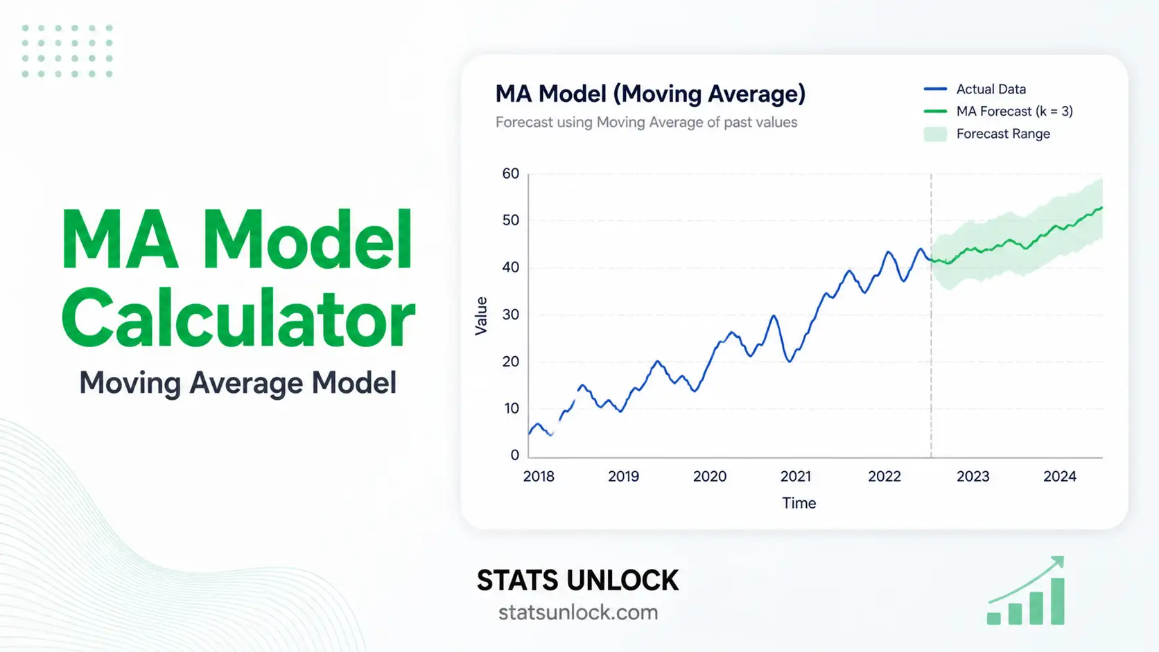
MA Model Calculator (Moving Average)
Fit a Moving Average MA(q) time series model online — get coefficients, residuals, ACF/PACF diagnostics, Ljung-Box white-noise test, AIC/BIC, forecasts, and APA-format reporting.
📥 Step 1 — Enter Time Series Data
Enter comma-separated values (default). Newlines are also accepted.
Click columns to select them as clusters, or skip columns you want to exclude. Use the toolbar to select all numeric columns at once or clear/skip everything.
⚙️ Step 2 — Configure MA Model
🧮 Technical Notes — Formulas & Methodology
MA(q) Model Formula
Yt = μ + εt + θ1·εt-1 + θ2·εt-2 + … + θq·εt-q
Where:
- Yt — value of the series at time t
- μ — mean of the series (constant)
- εt — white-noise error term at time t, with εt ~ N(0, σ²)
- θk — moving-average coefficient at lag k; carries the influence of the past shock εt-k into Yt
- q — order of the MA model (number of past errors used)
Estimation — Conditional Sum of Squares (CSS)
Given a candidate parameter vector (μ, θ1, …, θq), residuals are computed recursively assuming εt = 0 for t ≤ 0:
εt = (Yt − μ) − θ1·εt-1 − … − θq·εt-q
Coefficients minimize the conditional sum of squared residuals:
S(θ) = Σ εt² → minimize over θ
This calculator uses a numerical grid + Nelder-Mead-style coordinate descent to minimize S(θ), then computes σ̂² = S(θ̂) / (n − q − 1).
Information Criteria
AIC = n · ln(σ̂²) + 2·(q + 1)
BIC = n · ln(σ̂²) + (q + 1)·ln(n)
log-Lik ≈ −n/2 · [ln(2π) + ln(σ̂²) + 1]
Lower AIC and BIC indicate better trade-offs between fit and complexity.
Ljung-Box Q Statistic
Q(h) = n·(n+2) · Σk=1..h [ ρ̂k² / (n − k) ]
Where ρ̂k is the sample autocorrelation of residuals at lag k. Under H0 (residuals are white noise), Q ~ χ²(h − q). A non-significant p-value (p > α) indicates the MA(q) model has adequately captured the temporal structure.
Forecast Equation
An MA(q) forecast for h steps ahead is:
Ŷn+h = μ + Σk=h..q θk · εn+h−k (if h ≤ q)
Ŷn+h = μ (if h > q)
Beyond horizon q, the optimal forecast collapses to the series mean — a defining property of MA models.
📌 When to Use the MA Model
This free MA model calculator is designed for analysts, students, and researchers who need to fit an MA(q) moving average model to a stationary or weakly stationary time series. Choose this model when the data show short-memory shock dependence rather than long-running autoregressive behavior.
✓ Use MA(q) when:
- The sample ACF cuts off sharply after lag q while the PACF decays geometrically.
- The series is stationary (constant mean, constant variance, no trend).
- You expect short-lived random shocks to influence current and the next q periods, then dissipate.
- You need a parsimonious benchmark to compare against ARMA, ARIMA, or ETS models.
Examples
- Finance — Daily return series often follow MA(1) or MA(2) patterns reflecting short-lived information shocks.
- Retail — Sales after a one-week promotion may show MA(1) carry-over into the following week, then return to baseline.
- Climate — Daily temperature anomaly residuals after detrending typically follow low-order MA(q) processes.
- Quality control — Process error sequences in manufacturing where measurement shocks persist for q lags.
📖 How to Use This MA Model Calculator
STEP 1 — Enter Your Data
Three input options: paste/type comma-separated values (default), upload a CSV/Excel file and select a column, or fill the manual cells. The textarea expects a format like 52, 48, 55, 61, 47, …
STEP 2 — Choose a Sample Dataset
Five built-in datasets cover retail, finance, macroeconomics, web analytics, and climate. Dataset 1 (Monthly Retail Sales) loads on first render so the tool runs immediately.
STEP 3 — Configure MA Settings
Select the order q (1–5), alpha level (0.01, 0.05, 0.10), forecast horizon, and Ljung-Box lag. Start with MA(1) or MA(2) and only increase q if residuals still show autocorrelation.
STEP 4 — Run the Analysis
Click Run MA(q) Analysis. Coefficients, residuals, AIC, BIC, Ljung-Box Q, and the four diagnostic charts populate within a second.
STEP 5 — Read the Summary Cards
Green = good fit / coefficient significant; amber = borderline; red = problematic (e.g., Ljung-Box p < α indicates remaining autocorrelation).
STEP 6 — Read the Full Results Table
Each row shows a statistic with its value and a plain-language description. Pay special attention to coefficient SE / 95% CI: a CI containing zero suggests dropping that lag.
STEP 7 — Examine the Four Visualizations
Chart 1 = original series + fitted values + forecasts. Chart 2 = residuals over time (look for random scatter around zero). Charts 3 and 4 = ACF and PACF of residuals — both should sit inside the ±1.96/√n bands.
STEP 8 — Check Assumptions
The Assumption Check panel verifies stationarity (mean / variance), invertibility, and white-noise residuals. Yellow / red flags suggest differencing the series first or moving to ARIMA / SARIMA.
STEP 9 — Read the Interpretation
Five labelled report cards (APA, Thesis, Plain-Language, Conference, Pre-Reg) auto-fill with the live numbers. Click 📋 Copy to paste into your manuscript.
STEP 10 — Export Your Results
Use Download Doc for a plain-text report, or Download PDF to print/save a publication-ready PDF that includes all eight sections plus the StatsUnlock branding line.
❓ Frequently Asked Questions
Q1. What is an MA model and when should I use it?
A Moving Average MA(q) model expresses the current value of a time series as a linear combination of the current and past q white-noise error terms. Use MA(q) when the autocorrelation function (ACF) cuts off sharply after lag q while the partial autocorrelation function (PACF) decays gradually — that pattern indicates short-memory shock dependence rather than persistent autoregressive behavior. Common applications include short-horizon return modeling, post-promotion sales decay, and climate anomaly residuals.
Q2. What is a p-value, and how do I interpret it for an MA model?
For each coefficient θk, the p-value is the probability of observing an estimate at least as far from zero as the one we got, if the true coefficient were zero. A coefficient p-value < α (typically 0.05) means that lag of past error contributes meaningfully. For the Ljung-Box test on residuals, the interpretation flips: a non-significant p-value (p > α) is desirable because it means the residuals look like white noise.
Q3. What does statistical significance mean — and does it equal practical importance?
A coefficient can be statistically significant (p < α) but very small in magnitude, contributing little to forecast accuracy. Always inspect the magnitude of θ̂k, the size of σ̂² relative to the variance of the series, and the AIC reduction compared to the lower-order MA(q−1) model. Practical importance lives in those magnitudes, not the p-value alone.
Q4. How do I interpret the size of MA coefficients (Cohen-style benchmarks)?
MA coefficients are bounded by invertibility constraints. As rough benchmarks: |θ| < 0.20 is a small effect, 0.20–0.50 is moderate, and |θ| > 0.50 is large. A coefficient near the invertibility boundary (|θ| ≈ 1 for MA(1)) signals the model is straining and a different specification (e.g., differencing) might be more appropriate.
Q5. What assumptions does the MA model require, and what if my data violate them?
Key assumptions: (1) the series is stationary — constant mean and variance, no trend; (2) errors εt are independent, identically distributed with zero mean; (3) the model is invertible. If stationarity is violated, difference the series first (giving an ARIMA model). If residuals show heteroscedasticity, consider GARCH. If errors are non-Gaussian with heavy tails, robust standard errors or a different distribution should be used.
Q6. How large a sample do I need for an MA model to be reliable?
A practical floor is around 50 observations. With 100+ data points, MA(1) and MA(2) coefficient estimates become stable and standard errors tighten. Below 30, parameter estimates are unreliable regardless of how small the p-value looks; the AIC and BIC are still useful for ranking candidate orders, but treat individual coefficient inference cautiously.
Q7. What is the difference between MA and AR models?
An AR(p) model regresses the current value on past values of the series itself (Yt on Yt-1, …, Yt-p). An MA(q) model regresses the current value on past random errors (εt-1, …, εt-q). Diagnostic rule: ACF cuts off at lag q for MA(q); PACF cuts off at lag p for AR(p). When both decay gradually, an ARMA(p, q) blend is appropriate.
Q8. How do I report MA model results in APA 7th edition format?
Report the order, all coefficients with standard errors, residual variance σ̂², AIC, BIC, log-likelihood, and the Ljung-Box test on residuals. Example: An MA(1) model was fitted, θ1 = 0.42, SE = 0.11, σ̂² = 4.18, AIC = 218.6, BIC = 224.9; Ljung-Box on residuals indicated no remaining autocorrelation, Q(10) = 8.21, p = .61. Section 2.7 of this page provides five fully filled-in templates.
Q9. Can I use this calculator for my published research or university assignment?
Yes for educational use, course assignments, and exploratory analysis. For peer-reviewed publication, cross-validate the result with a mature library — R (forecast, stats), Python (statsmodels), or a commercial package — because those use full maximum-likelihood with state-space Kalman filtering. Cite this tool as: STATS UNLOCK. (2025). MA Model calculator. Retrieved from https://statsunlock.com.
Q10. What should I do if the Ljung-Box test on residuals is significant?
A significant Ljung-Box (p < α) means residual autocorrelation remains — the MA(q) model has not fully captured the temporal dependence. Try (1) increasing q by one, (2) adding an AR component (ARMA(p, q)), (3) differencing the series if a trend is visible (ARIMA), or (4) modeling seasonality with SARIMA if a periodic pattern shows in the ACF. Always re-run the Ljung-Box on the new residuals to confirm white-noise behavior.
📚 References
The following references support the methodology of this MA model calculator, the moving average model time series example logic, and the MA model interpretation guide used throughout this page.
- Box, G. E. P., Jenkins, G. M., Reinsel, G. C., & Ljung, G. M. (2015). Time Series Analysis: Forecasting and Control (5th ed.). Wiley. link
- Brockwell, P. J., & Davis, R. A. (2016). Introduction to Time Series and Forecasting (3rd ed.). Springer. https://doi.org/10.1007/978-3-319-29854-2
- Hamilton, J. D. (1994). Time Series Analysis. Princeton University Press. link
- Hyndman, R. J., & Athanasopoulos, G. (2021). Forecasting: Principles and Practice (3rd ed.). OTexts. https://otexts.com/fpp3/
- Ljung, G. M., & Box, G. E. P. (1978). On a measure of lack of fit in time series models. Biometrika, 65(2), 297–303. https://doi.org/10.1093/biomet/65.2.297
- Akaike, H. (1974). A new look at the statistical model identification. IEEE Transactions on Automatic Control, 19(6), 716–723. https://doi.org/10.1109/TAC.1974.1100705
- Schwarz, G. (1978). Estimating the dimension of a model. Annals of Statistics, 6(2), 461–464. https://doi.org/10.1214/aos/1176344136
- Shumway, R. H., & Stoffer, D. S. (2017). Time Series Analysis and Its Applications (4th ed.). Springer. https://doi.org/10.1007/978-3-319-52452-8
- Cryer, J. D., & Chan, K.-S. (2008). Time Series Analysis: With Applications in R (2nd ed.). Springer. https://doi.org/10.1007/978-0-387-75959-3
- Tsay, R. S. (2010). Analysis of Financial Time Series (3rd ed.). Wiley. link
- Hyndman, R. J., & Khandakar, Y. (2008). Automatic time series forecasting: The forecast package for R. Journal of Statistical Software, 27(3), 1–22. https://doi.org/10.18637/jss.v027.i03
- R Core Team. (2024). R: A Language and Environment for Statistical Computing. R Foundation for Statistical Computing. https://www.r-project.org/
- Seabold, S., & Perktold, J. (2010). statsmodels: Econometric and statistical modeling with Python. Proceedings of the 9th Python in Science Conference. https://www.statsmodels.org/
- Hipel, K. W., & McLeod, A. I. (1994). Time Series Modelling of Water Resources and Environmental Systems. Elsevier. link
- American Psychological Association. (2020). Publication Manual of the American Psychological Association (7th ed.). link


