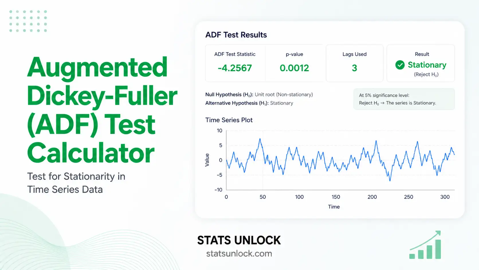
⚡ Augmented Dickey-Fuller Test Calculator
Free online ADF unit root test — check stationarity of any time series, get ADF statistic, p-value, critical values, and publication-ready results instantly.
| t | Value |
|---|
🔍 Interpretation of Results & How to Write Up in Research
🧮 Technical Notes & Formulas
The Augmented Dickey-Fuller test uses the following regression equations, depending on the model specification:
📖 How to Use This ADF Test Calculator — Step-by-Step Guide
Paste values into the text area (comma-separated or one per line), upload a CSV/Excel file and click a column, or use the manual grid. Values must be numeric and in time order (oldest first). Minimum 10 observations required.
Click the editable Series Name field and type a meaningful label. This name will appear on charts and in the downloaded report. Example: "CPI_Monthly", "Rainfall_mm_1990-2020", "Population_Count".
Select from five built-in datasets — GDP growth, temperature, wildlife population index, stock price, or rainfall — to explore how the tool works before using your own data. Each illustrates different stationarity patterns.
Choose α = 0.05 for standard research (default). Use α = 0.01 for strict hypothesis testing or financial applications. Use α = 0.10 for exploratory or pilot studies. The critical values displayed adjust automatically.
"With Constant" is the most common choice and handles series with non-zero means. Select "Constant + Trend" if the series plots show a clear upward or downward slope. "No Constant" is rarely used in practice — only for series that genuinely fluctuate around zero.
AIC (default) balances fit and parsimony and is best for most applications. BIC is more conservative (fewer lags) and preferred for small samples or where parsimony is important. "Fixed Lag" lets you specify exactly p lags based on theory or prior studies.
The calculator runs OLS regression for each candidate lag (up to the Schwert maximum), selects the best lag by the chosen criterion, computes the ADF τ statistic, and applies MacKinnon (1994) critical values and p-value approximation.
A green banner confirms the series is stationary (I(0)) — safe to use directly in ARIMA, regression, and other models. A red banner means non-stationary (I(1)) — apply first-order differencing (ΔYt = Yt − Yt-1) and re-run.
Chart 1 shows the raw series (look for trends and structural shifts). Chart 2 shows the first-differenced series (should look stationary). Chart 3 shows the ACF (should decay to near-zero quickly for a stationary series). Chart 4 compares your ADF τ to the 1%, 5%, and 10% critical values visually.
Use the five write-up cards — APA 7th, Thesis, Plain Language, Structured Abstract, Pre-Registration — to copy formatted results directly into your manuscript. Download the full report as a .txt file or print to PDF for your records and supplementary materials.
❓ Frequently Asked Questions
What is the Augmented Dickey-Fuller (ADF) test?
What is the null hypothesis of the ADF test?
How do I interpret the ADF statistic?
How many lags should I use in the ADF test?
What model specification should I choose?
What do I do if my time series is non-stationary?
What is the difference between the ADF test and KPSS test?
Can I use this ADF calculator for ecological or biological time series?
How do I report ADF test results in APA 7th edition?
What are MacKinnon critical values and why are they different from standard t-values?
🗺 When to Use the Augmented Dickey-Fuller Test
This free Augmented Dickey-Fuller test calculator is designed for researchers, analysts, and students who need to check stationarity as part of a time series analysis workflow. Use the ADF test when:
- You plan to fit an ARIMA, SARIMA, or VAR model and need to determine the differencing order (d).
- You are testing for cointegration (Engle-Granger two-step) and need to confirm each series is I(1) before testing for a long-run relationship.
- You are analysing economic or financial time series (GDP, inflation, exchange rates, stock prices, interest rates).
- You are pre-processing ecological, environmental, or biological time series (population indices, NDVI, rainfall, temperature) before fitting dynamic models.
- You need to avoid the spurious regression problem: regressing one non-stationary series on another produces misleadingly high R² values and invalid t-statistics.
- A reviewer, thesis supervisor, or journal requires you to document stationarity testing as part of your time series methods section.
- You want to determine the integration order of variables before including them in a distributed lag (ARDL) or error-correction model (ECM).
Model Specification Decision Guide
| Situation | Recommended Model | Rationale |
|---|---|---|
| Series with no trend; mean ≠ 0 | Constant only | Most common default; accounts for non-zero mean without over-specifying |
| Series with clear upward or downward trend | Constant + Trend | Prevents spurious rejection due to deterministic trend component |
| Series fluctuating around zero | No Constant | Parsimonious; rarely appropriate in real-world data |
| Uncertain — inspect plot first | Try Constant, then Constant + Trend | Visual inspection + information criteria (AIC) help guide the choice |
🏁 Conclusion
The Augmented Dickey-Fuller (ADF) test is one of the most fundamental tools in time series analysis. Before building any forecasting or structural model — ARIMA, VAR, cointegration, or error-correction — you must first confirm whether your series is stationary. A non-stationary series violates the assumptions of most standard models, producing spurious regression results, misleading forecasts, and invalid hypothesis tests (Granger & Newbold, 1974). The ADF test gives you an objective, peer-reviewed statistical criterion for making that determination.
This free ADF test calculator handles the complete workflow: automatic lag selection via AIC or BIC using the Schwert (1989) maximum lag rule, three model specifications (no constant, constant only, constant + trend), MacKinnon (1994) critical values and p-value approximation, and four diagnostic charts that make the results visual and easy to communicate. You do not need R, Python, Stata, or specialist econometrics software — the tool runs entirely in your browser and produces publication-ready output instantly.
When the ADF test rejects the null hypothesis (p < α), your series is stationary — you can proceed directly to model fitting without differencing. When it fails to reject (p ≥ α), apply first-order differencing and re-run the test. Most real-world series — economic indicators, wildlife population counts, climate variables — are integrated of order one (I(1)), so one round of differencing is usually sufficient to achieve stationarity.
Always complement ADF results with visual inspection of the raw time series plot and the ACF. If your series contains a structural break (policy shift, ecological disturbance, market crash), consider the Zivot-Andrews (1992) test, which allows for one unknown break point — the ADF test may incorrectly fail to reject H₀ in the presence of structural breaks. For multiple series, consider the Im-Pesaran-Shin (2003) panel unit root test.
Reporting transparently is central to reproducible time series research. Use the five write-up templates in the Interpretation panel above — APA 7th edition, Thesis, Plain Language, Structured Abstract, and Pre-Registration — to produce correctly formatted results for any journal or institutional requirement. Always report the ADF statistic, lag count, model specification, and exact MacKinnon p-value in your methods section so readers can fully evaluate and replicate your analysis.
📚 References
The following peer-reviewed references support the Augmented Dickey-Fuller test methodology, unit root testing theory, lag selection criteria, and stationarity analysis described in this augmented Dickey-Fuller test calculator and unit root test guide.
- Dickey, D. A., & Fuller, W. A. (1979). Distribution of the estimators for autoregressive time series with a unit root. Journal of the American Statistical Association, 74(366), 427–431. https://doi.org/10.2307/2286348
- Dickey, D. A., & Fuller, W. A. (1981). Likelihood ratio statistics for autoregressive time series with a unit root. Econometrica, 49(4), 1057–1072. https://doi.org/10.2307/1912517
- MacKinnon, J. G. (1994). Approximate asymptotic distribution functions for unit-root and cointegration tests. Journal of Business & Economic Statistics, 12(2), 167–176. https://doi.org/10.1080/07350015.1994.10510005
- MacKinnon, J. G. (2010). Critical values for cointegration tests (Queen’s Economics Department Working Paper No. 1227). Queen’s University. https://ideas.repec.org/p/qed/wpaper/1227.html
- Schwert, G. W. (1989). Tests for unit roots: A Monte Carlo investigation. Journal of Business & Economic Statistics, 7(2), 147–159. https://doi.org/10.1080/07350015.1989.10509723
- Kwiatkowski, D., Phillips, P. C. B., Schmidt, P., & Shin, Y. (1992). Testing the null hypothesis of stationarity against the alternative of a unit root. Journal of Econometrics, 54(1–3), 159–178. https://doi.org/10.1016/0304-4076(92)90104-Y
- Said, S. E., & Dickey, D. A. (1984). Testing for unit roots in autoregressive-moving average models of unknown order. Biometrika, 71(3), 599–607. https://doi.org/10.1093/biomet/71.3.599
- Elliott, G., Rothenberg, T. J., & Stock, J. H. (1996). Efficient tests for an autoregressive unit root. Econometrica, 64(4), 813–836. https://doi.org/10.2307/2171846
- Phillips, P. C. B., & Perron, P. (1988). Testing for a unit root in time series regression. Biometrika, 75(2), 335–346. https://doi.org/10.1093/biomet/75.2.335
- Zivot, E., & Andrews, D. W. K. (1992). Further evidence on the great crash, the oil-price shock, and the unit-root hypothesis. Journal of Business & Economic Statistics, 10(3), 251–270. https://doi.org/10.1080/07350015.1992.10509904
- Hamilton, J. D. (1994). Time series analysis. Princeton University Press. https://press.princeton.edu/books
- Enders, W. (2014). Applied econometric time series (4th ed.). Wiley. https://www.wiley.com
- Granger, C. W. J., & Newbold, P. (1974). Spurious regressions in econometrics. Journal of Econometrics, 2(2), 111–120. https://doi.org/10.1016/0304-4076(74)90034-7
- Akaike, H. (1974). A new look at the statistical model identification. IEEE Transactions on Automatic Control, 19(6), 716–723. https://doi.org/10.1109/TAC.1974.1100705
- Im, K. S., Pesaran, M. H., & Shin, Y. (2003). Testing for unit roots in heterogeneous panels. Journal of Econometrics, 115(1), 53–74. https://doi.org/10.1016/S0304-4076(03)00092-7


