Exploratory Factor Analysis
Calculator
Uncover latent factors in your data — enter variables, run EFA, and get factor loadings, KMO, scree plot, communalities, and full APA reporting templates instantly. No software required.
Step 1 — Enter Your Variable Data
Enter each variable's observed scores as comma-separated numbers, e.g.: 52, 48, 55, 61, 47, 53, 58, 60, ... | Each variable = one survey item / scale indicator. All variables must have equal observation counts (minimum 5).
Supports .csv, .txt, .xlsx, .xls — headers detected automatically. Click column buttons to select which columns become EFA variables. Each selected column = one variable (row of scores).
Type values directly into the grid. Each row = one observation; each column = one variable.
Step 2 — Configure EFA Settings
🔬 Formulas & Technical Notes
🎯 When to Use Exploratory Factor Analysis
EFA is appropriate when you suspect multiple observed variables share underlying latent constructs and you want the data to reveal the factor structure — without pre-specifying it. It is the standard first step in scale development, instrument validation, and any domain where you need to reduce many correlated variables to a smaller set of meaningful dimensions.
- ✔You have ≥ 3 observed continuous or ordered variables (Likert scales ≥ 5 points are acceptable)
- ✔Variables are meaningfully correlated (KMO ≥ 0.60; Bartlett's test p < α)
- ✔You have ≥ 5 observations per variable (ideally n ≥ 100 for stable solutions)
- ✔Your goal is to discover the latent structure — not confirm a pre-specified model
- ✔You are developing or refining a multi-item measurement scale
- ✗Do NOT use if you already have a confirmed factor structure → use CFA instead
- ✗Do NOT use if variables are purely binary → use tetrachoric correlations + IRT
- ✗Do NOT use if your goal is dimension reduction only (not construct measurement) → use PCA
- ✗Do NOT use with n < 50 — factor solutions will be unstable and unreliable
Real-World Use Cases
EFA Decision Tree
Multiple correlated variables → Goal: reduce dimensions, maximise variance → PCA
Confirmed theory-driven factor structure → Test model fit → CFA
Binary items (0/1) → Use polychoric correlations → EFA with polychoric R
Categorical items + factor structure → Factor mixture models
After EFA finds factor structure → Validate on new sample → CFA next step
📖 How to Use This EFA Calculator — Step-by-Step Guide
Prepare Your Data
Each "variable" is one measured item (e.g., one survey question, one test score). Gather your observations for each item. If you have a data file (.csv, .xlsx), use the Upload tab — no manual typing needed.
Enter Variable Names
Click the grey name field next to each variable and type a meaningful label (e.g., Q1_Anxiety, Extraversion_Item3, SleepQuality). These labels appear in the factor loadings table. Default names are "Variable 1", "Variable 2", etc.
Enter Observed Scores
In the text area next to each variable name, type or paste the scores — comma-separated, e.g.: 52, 48, 55, 61, 47, 53, 58, 60. All variables must have the same number of values. Load one of 5 built-in sample datasets to try the tool immediately.
Upload CSV / Excel (Alternative)
Switch to the Upload tab and drag-drop or browse to your file. After loading, column buttons appear. Click each column you want to include as an EFA variable — it will turn green. Then click "Use Selected Columns".
Configure Settings
Choose extraction method (PAF recommended for EFA), rotation (Varimax is standard for orthogonal structure), and factor retention rule (Kaiser criterion is the most common starting point). Set the loading threshold — 0.40 is standard in most fields.
Run the Analysis
Click the green "Run Exploratory Factor Analysis" button. Results appear immediately below — no page reload.
Read the Summary Cards
Six cards show KMO (green = ≥ 0.80 meritorious), Bartlett's χ² with p-value, number of factors retained, total variance explained, minimum communality, and sample size. Check for green indicators before interpreting factor structure.
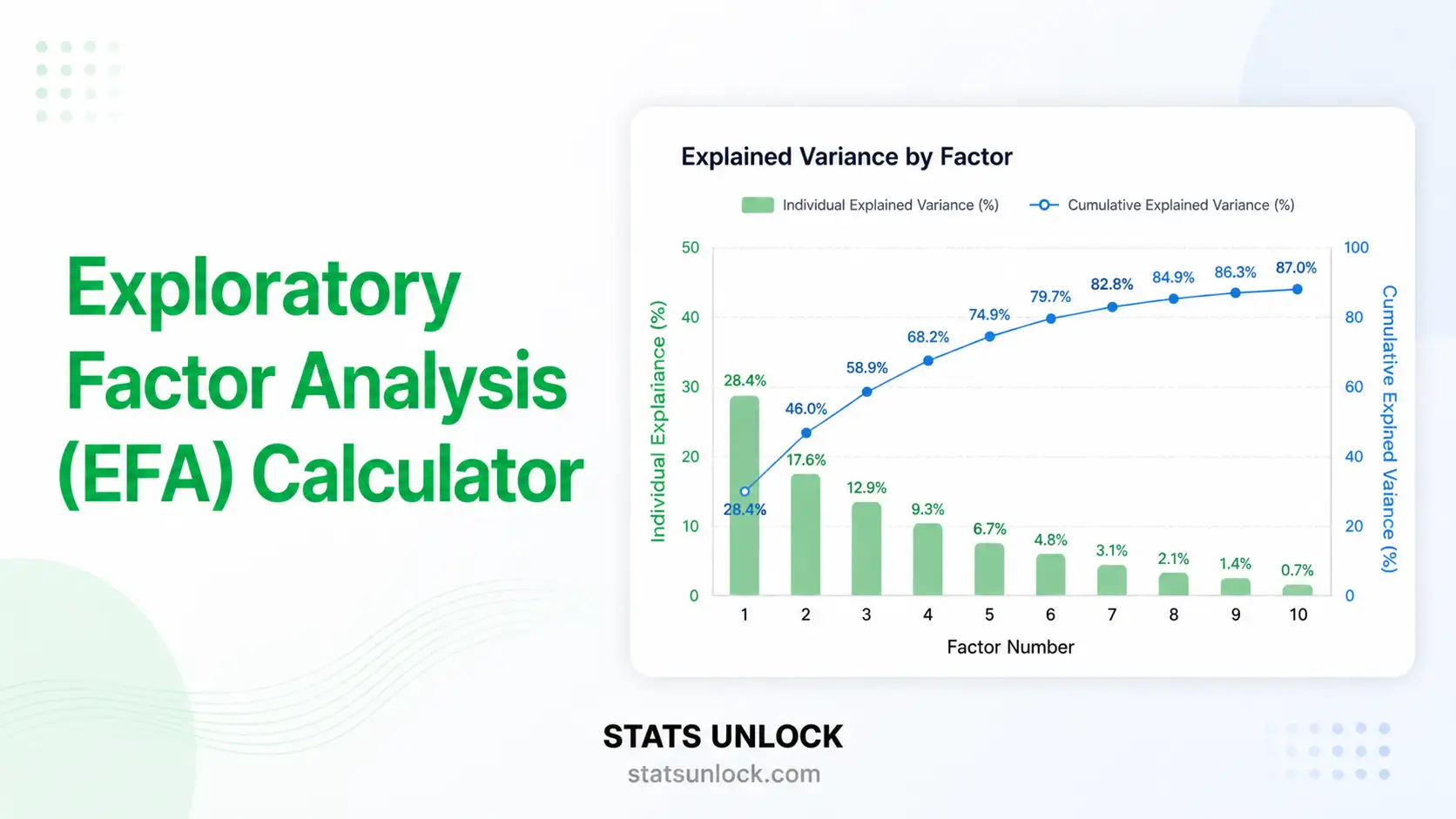
Examine the Scree Plot (Chart 1)
The scree plot shows eigenvalues for each factor in descending order. Look for the "elbow" — the bend after which the line flattens. Factors above the elbow are worth retaining. The red dashed line marks eigenvalue = 1 (Kaiser criterion).
Interpret Factor Loadings (Chart 3 + Table)
The loadings table shows how strongly each variable relates to each factor. Green cells (≥ 0.70) indicate strong relationships; amber cells (≥ threshold) indicate salient loadings. For clean simple structure, each variable should load high on ONE factor and near zero on all others.
Export and Report
Copy from any of the 5 reporting templates (APA 7th, Thesis, Plain Language, Abstract, Pre-Registration). Download a full .txt report or PDF for your records. Cite this tool as: StatsUnlock (2025). Exploratory Factor Analysis Calculator. Retrieved from statsunlock.com.
❓ Frequently Asked Questions
What is exploratory factor analysis (EFA) and when should I use it?
Exploratory factor analysis is a statistical method used to identify the latent (hidden) structure underlying a set of observed variables. It answers the question: "How many unobserved constructs explain the correlations among these variables?" Use EFA when developing a new scale, when you have no strong prior theory about factor structure, or when you want the data to reveal its own structure — before moving to confirmatory factor analysis (CFA) to test that structure on new data.
How many factors should I retain?
No single method is universally best. Use multiple criteria together: (1) Kaiser criterion — retain factors with eigenvalue > 1 (simple but can over-extract in large samples); (2) Scree plot — retain factors above the "elbow" in the eigenvalue plot; (3) Parallel analysis — compare your eigenvalues to those from random data of the same dimensions (generally most accurate); (4) Interpretability — the factor structure should make theoretical sense. If criteria disagree, examine solutions with ±1 factor and choose the most interpretable.
What is KMO and what value do I need?
The Kaiser-Meyer-Olkin (KMO) measure assesses sampling adequacy — whether the pattern of correlations among variables is compact enough for factor analysis to produce distinct, reliable factors. KMO benchmarks: ≥ 0.90 = Marvelous, 0.80–0.89 = Meritorious, 0.70–0.79 = Middling, 0.60–0.69 = Mediocre, 0.50–0.59 = Miserable, < 0.50 = Unacceptable. A KMO ≥ 0.70 is typically required before proceeding with EFA.
What is the difference between EFA and PCA?
EFA and PCA look similar but have fundamentally different goals. EFA assumes observed variables are caused by underlying latent factors — it separates common variance (shared among variables) from unique variance and error. It is a causal model for construct measurement. PCA creates linear composites that maximally explain total variance (common + unique + error) — it is purely a data-reduction technique with no causal assumptions. Use EFA when you believe latent constructs drive the correlations; use PCA when you only want to reduce dimensions efficiently.
What is communality and what does a low value mean?
Communality (h²) is the proportion of a variable's total variance explained by the retained factors. Values range from 0 (no shared variance) to 1 (all variance is shared). A communality of 0.65 means 65% of that variable's variance is captured by the factor solution. Low communality (h² < 0.30) suggests a variable does not fit well with the other variables and may need to be removed or that more factors should be retained. Very high communalities (> 0.95) may indicate multicollinearity issues.
What is Varimax rotation and when should I use it?
Varimax is an orthogonal rotation that maximises the variance of squared loadings within each factor. It pushes loadings toward 0 or ±1, making simple structure clearer: each variable tends to load highly on one factor and near zero on others. Use Varimax when you have theoretical reason to believe the underlying constructs are independent (uncorrelated). If factors are likely correlated (e.g., anxiety and depression), use an oblique rotation like Promax or Oblimin instead — these are available in R's psych package or SPSS.
What sample size do I need for EFA?
Rules of thumb vary: a common minimum is n ≥ 5 per variable, with n ≥ 100 as an absolute minimum for stable results and n ≥ 200 preferred. MacCallum et al. (1999) showed that adequate sample size depends on communalities and factor overdetermination: with high communalities (h² > 0.60) and well-determined factors (4+ salient loadings per factor), n = 100–150 may suffice. With low communalities or poorly defined factors, n ≥ 300 is recommended. Always report sample size and communalities alongside your EFA results.
How do I report EFA results in APA 7th edition format?
A complete APA 7 EFA report should include: (1) extraction method (e.g., principal axis factoring), (2) rotation method (e.g., Varimax), (3) factor retention criteria and number of factors, (4) KMO value, (5) Bartlett's test statistics: χ², df, and p-value, (6) eigenvalues and cumulative variance for each retained factor, (7) loading threshold used for interpretation, and (8) a factor loading matrix table. Example: "An EFA using principal axis factoring with Varimax rotation revealed a 2-factor solution (KMO = .82, Bartlett's χ²(10) = 95.3, p < .001) explaining 64.2% of variance (Factor 1: 42.1%, Factor 2: 22.1%)." Use the auto-filled templates below for complete reporting examples.
My factor solution is hard to interpret — what should I do?
Common causes of poor simple structure: (1) Wrong number of factors — try ±1 factor; (2) Cross-loading items — items loading ≥ threshold on two or more factors are ambiguous; consider removing them; (3) Wrong rotation — if factors are theoretically correlated, switch from Varimax to Promax/Oblimin; (4) Small sample — solutions with n < 100 are often unstable; (5) Inadequate measure diversity — you may need more items per expected factor (aim for 4+ items per factor). Always examine the scree plot alongside the Kaiser criterion, and consider parallel analysis for a more objective retention decision.
Can I use this tool for academic research or assignments?
Yes — this tool performs standard EFA computations (correlation matrix, eigendecomposition, Varimax rotation, KMO, Bartlett's test) consistent with methods used in R (psych package), SPSS, and SAS. For peer-reviewed publications, we recommend verifying results with dedicated statistical software and reporting the verification. For coursework, theses, and preliminary research, this tool provides complete, citable results. Cite as: StatsUnlock (2025). Exploratory Factor Analysis Calculator. Retrieved from https://statsunlock.com/calculators/exploratory-factor-analysis-calculator/
References
The following references support the exploratory factor analysis methods, formulas, and interpretation guidelines used in this EFA calculator. All in APA 7th edition format.
- Cattell, R. B. (1966). The scree test for the number of factors. Multivariate Behavioral Research, 1(2), 245–276. https://doi.org/10.1207/s15327906mbr0102_10
- Fabrigar, L. R., Wegener, D. T., MacCallum, R. C., & Strahan, E. J. (1999). Evaluating the use of exploratory factor analysis in psychological research. Psychological Methods, 4(3), 272–299. https://doi.org/10.1037/1082-989X.4.3.272
- Floyd, F. J., & Widaman, K. F. (1995). Factor analysis in the development and refinement of clinical assessment instruments. Psychological Assessment, 7(3), 286–299. https://doi.org/10.1037/1040-3590.7.3.286
- Hair, J. F., Black, W. C., Babin, B. J., & Anderson, R. E. (2019). Multivariate data analysis (8th ed.). Cengage Learning. https://www.cengage.com/c/multivariate-data-analysis-8e-hair/
- Hayton, J. C., Allen, D. G., & Scarpello, V. (2004). Factor retention decisions in exploratory factor analysis: A tutorial on parallel analysis. Organizational Research Methods, 7(2), 191–205. https://doi.org/10.1177/1094428104263675
- Horn, J. L. (1965). A rationale and test for the number of factors in factor analysis. Psychometrika, 30(2), 179–185. https://doi.org/10.1007/BF02289447
- Kaiser, H. F. (1960). The application of electronic computers to factor analysis. Educational and Psychological Measurement, 20(1), 141–151. https://doi.org/10.1177/001316446002000116
- Kaiser, H. F. (1974). An index of factorial simplicity. Psychometrika, 39(1), 31–36. https://doi.org/10.1007/BF02291575
- MacCallum, R. C., Widaman, K. F., Zhang, S., & Hong, S. (1999). Sample size in factor analysis. Psychological Methods, 4(1), 84–99. https://doi.org/10.1037/1082-989X.4.1.84
- Mundfrom, D. J., Shaw, D. G., & Ke, T. L. (2005). Minimum sample size recommendations for conducting factor analyses. International Journal of Testing, 5(2), 159–168. https://doi.org/10.1207/s15327574ijt0502_4
- Preacher, K. J., & MacCallum, R. C. (2003). Repairing Tom Swift's electric factor analysis machine. Understanding Statistics, 2(1), 13–43. https://doi.org/10.1207/S15328031US0201_02
- R Core Team. (2024). R: A language and environment for statistical computing. R Foundation for Statistical Computing. https://www.R-project.org/
- Revelle, W. (2024). psych: Procedures for psychological, psychometric, and personality research. R package version 2.4.3. https://CRAN.R-project.org/package=psych
- Tabachnick, B. G., & Fidell, L. S. (2019). Using multivariate statistics (7th ed.). Pearson. https://www.pearson.com/en-us/subject-catalog/p/using-multivariate-statistics/
- Zwick, W. R., & Velicer, W. F. (1986). Comparison of five rules for determining the number of components to retain. Psychological Bulletin, 99(3), 432–442. https://doi.org/10.1037/0033-2909.99.3.432


