ARIMA Model Calculator
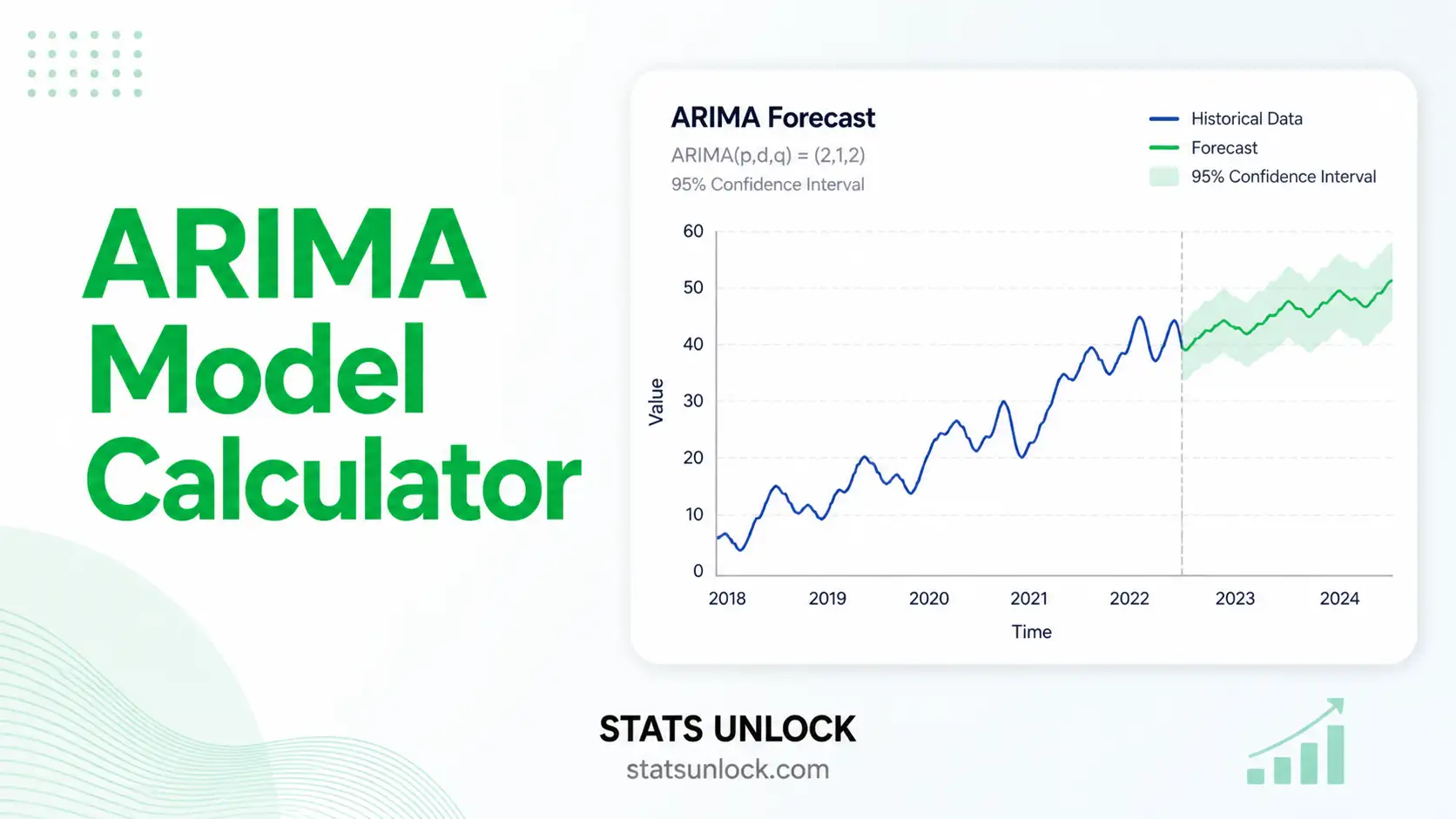
Fit an ARIMA(p, d, q) model to any time series — get parameter estimates, ACF / PACF, residual diagnostics, AIC / BIC, and a forecast with 95% confidence intervals.
📈 Series + Forecast
🔁 ACF (Lag 1–20)
📊 PACF (Lag 1–20)
🎯 Residuals
📥 1. Enter Your Time Series
Add multiple time-series clusters/groups. Each cluster gets fit independently. The group name is editable.
⚙️ Model settings
📊 2. Model Results
Results will appear here after you click Run ARIMA Analysis.
🧠 3. Interpretation Results & How to Write Your Results
📖 Detailed Interpretation Results
▶ Run the analysis above to populate the interpretation with your computed values.
✍️ How to Write Your Results in Research (5 Examples)
🏁 4. Conclusion
▶ Run the analysis to generate the full study conclusion.
🧮 5. Technical Notes & Formulas
A. Formulas
ARIMA(p, d, q) model. Let yt be the original series and let ∇dyt be the d-th difference. Then:
- yt — observed value at time t
- ∇dyt — d-th difference, e.g. ∇yt = yt − yt−1
- c — drift / intercept term
- φi — autoregressive (AR) coefficient at lag i
- θj — moving-average (MA) coefficient at lag j
- εt ~ WN(0, σ²) — white-noise error
ACF at lag k:
PACF at lag k is the last coefficient φkk from the Yule–Walker / Durbin–Levinson recursion fitting an AR(k) model to the series.
AIC and BIC for the fitted model:
Ljung–Box Q statistic on residuals (lag h):
Forecast variance. For an ARIMA(p, d, q) forecast at horizon h, the variance grows with h via the MA(∞) representation: σ²h = σ² · Σj=0..h−1 ψj². The 95% prediction interval is ŷn+h ± 1.96·√σ²h.
B. Notes
- ADF test should reject at α = 0.05 after differencing (i.e. the d-th differenced series should be stationary).
- Residuals should be white noise: a non-significant Ljung–Box result is desired.
- Compare AIC and BIC across competing (p, d, q) candidates — lower is better.
- This calculator uses an OLS-style approximation to the Box–Jenkins MLE for the AR and MA coefficients, suitable for educational and exploratory use.
📌 6. When to Use the ARIMA Model
ARIMA is appropriate when your data are an evenly spaced time series, show autocorrelation, and you want short- to medium-horizon forecasts that account for past values and past forecast errors.
Decision checklist
- ✅ Univariate time series with regular intervals
- ✅ At least ~50 observations
- ✅ Series can be made stationary by differencing (d = 0, 1, or 2)
- ✅ ACF / PACF show interpretable autocorrelation structure
- ❌ Strong seasonal pattern → use SARIMA(p,d,q)(P,D,Q)s instead
- ❌ Multiple correlated series → consider VAR
- ❌ Non-linear or volatility-driven dynamics → consider ARCH / GARCH or state-space models
Real-world examples
- Economics — forecasting quarterly GDP growth or monthly inflation rates.
- Retail / Sales — projecting next quarter's revenue from monthly sales history.
- Energy — predicting daily electricity demand or wind-power output.
- Public health / Ecology — modelling weekly disease incidence or wildlife counts.
Sample-size guidance
- Minimum ~50 observations for a stable ARIMA(p,d,q) fit.
- Forecast horizon should not exceed ~25% of the historical length.
- Use cross-validation or hold-out evaluation (RMSE, MAPE) for honest performance estimates.
📘 7. How to Use This Tool — Step by Step
- Enter your data — paste comma-separated values (default), upload a CSV/Excel, or add multiple clusters in the Multi-series tab.
- Choose a sample dataset — five built-in datasets cover trend, seasonality, finance, traffic, and economics.
- Set the orders (p, d, q) — start with d from the differencing required for stationarity; pick p from the PACF cut-off, q from the ACF cut-off.
- Or use Auto order — the tool searches up to (3,2,3) and picks the model with the lowest AIC.
- Click Run ARIMA Analysis — model fits in the browser, no server, no upload of your data.
- Read the model summary cards — model order, log-likelihood, AIC, BIC, residual SD, Ljung-Box p-value.
- Inspect the four plots — series + forecast, ACF, PACF, residuals.
- Check residuals — Ljung-Box p > 0.05 indicates the model has captured the autocorrelation structure.
- Read the interpretation block — auto-filled paragraphs translate the numbers into plain English.
- Export — Download Doc (text) or Download PDF (print-ready report).
❓ 8. Frequently Asked Questions
Q1. What is the ARIMA model and when should I use it?
ARIMA — AutoRegressive Integrated Moving Average — is a classical time-series model that combines past values (AR), differencing for stationarity (I), and past forecast errors (MA). Use it when your data are evenly spaced, show autocorrelation, and you want short- to medium-term forecasts with reasonable interpretability.
Q2. What do p, d, and q mean in ARIMA(p,d,q)?
p is the AR order — how many past values feed into today's value. d is the number of times you differenced the series to make it stationary. q is the MA order — how many past forecast errors enter the model. A series like ARIMA(1,1,1) uses one AR term, one differencing, and one MA term.
Q3. How do I choose the right (p, d, q)?
Choose d so the d-th differenced series looks stationary (flat mean, constant variance, ADF rejects the unit root). Then use the ACF and PACF: a sharp PACF cut-off at lag p suggests AR(p); a sharp ACF cut-off at lag q suggests MA(q). Compare candidates by AIC/BIC and verify residuals are white noise (Ljung–Box).
Q4. What does the p-value mean for the Ljung–Box test?
The Ljung–Box test asks: are the residuals white noise? A high p-value (typically p > 0.05) means we cannot reject "no autocorrelation in residuals" — the model has adequately captured the temporal structure. A small p-value warns that something is still left in the residuals.
Q5. Does my time series need to be stationary?
The differenced series — that is, ∇dyt — must be approximately stationary in mean and variance. Trend or non-constant variance violates ARMA's assumptions, which is why the "I" (integration / differencing) step exists. Use ADF or KPSS to check, and apply log/Box–Cox transforms when variance grows with the level.
Q6. What is the difference between ARIMA and SARIMA?
ARIMA models non-seasonal patterns. SARIMA adds seasonal terms (P, D, Q) at period s — for example monthly data with yearly seasonality is often modelled as SARIMA(1,1,1)(1,1,1)12. If your ACF shows large spikes at lag 12 or 24, you probably need SARIMA, not plain ARIMA.
Q7. What is AIC vs BIC, and which should I trust?
Both penalise model complexity, but BIC penalises more strongly. For pure forecasting accuracy, AIC often performs slightly better; for parsimony and small samples, BIC is preferred. In practice, report both — and confirm with residual diagnostics and out-of-sample MAPE/RMSE.
Q8. How many data points do I need for ARIMA?
At least 50 observations for a stable fit, more for higher-order models. For seasonal data (SARIMA), aim for 4–5 full seasonal cycles. Forecast horizon should be much smaller than the historical length — forecasting 24 months from 30 months of history is unwise.
Q9. How do I report ARIMA results in a paper?
State the chosen order (p,d,q), parameter estimates with standard errors and significance, log-likelihood, AIC, BIC, residual SD, the Ljung–Box statistic and p-value, and out-of-sample forecast accuracy (RMSE, MAPE) where applicable. The Section 3 examples on this page provide ready-to-paste templates.
Q10. Can I use this calculator for my thesis or publication?
Yes for exploratory analysis and learning. For the final manuscript, replicate in R (forecast, fable), Python (statsmodels, pmdarima) or Stata, and cite the software and package version. STATS UNLOCK is suitable as an educational reference and as a quick check during model selection.
📚 9. References
The following references support the statistical methods used in this ARIMA model calculator, covering time series forecasting, ACF / PACF interpretation, and best practices in Box–Jenkins methodology.
- Box, G. E. P., & Jenkins, G. M. (1970). Time Series Analysis: Forecasting and Control. Holden-Day.
- Box, G. E. P., Jenkins, G. M., Reinsel, G. C., & Ljung, G. M. (2015). Time Series Analysis: Forecasting and Control (5th ed.). Wiley. https://doi.org/10.1002/9781118619193
- Hyndman, R. J., & Athanasopoulos, G. (2021). Forecasting: Principles and Practice (3rd ed.). OTexts. https://otexts.com/fpp3/
- Brockwell, P. J., & Davis, R. A. (2016). Introduction to Time Series and Forecasting (3rd ed.). Springer. https://doi.org/10.1007/978-3-319-29854-2
- Hyndman, R. J., & Khandakar, Y. (2008). Automatic time series forecasting: The forecast package for R. Journal of Statistical Software, 27(3), 1–22. https://doi.org/10.18637/jss.v027.i03
- Ljung, G. M., & Box, G. E. P. (1978). On a measure of lack of fit in time series models. Biometrika, 65(2), 297–303. https://doi.org/10.1093/biomet/65.2.297
- Dickey, D. A., & Fuller, W. A. (1979). Distribution of the estimators for autoregressive time series with a unit root. Journal of the American Statistical Association, 74(366a), 427–431. https://doi.org/10.1080/01621459.1979.10482531
- Kwiatkowski, D., Phillips, P. C. B., Schmidt, P., & Shin, Y. (1992). Testing the null hypothesis of stationarity against the alternative of a unit root. Journal of Econometrics, 54(1–3), 159–178. https://doi.org/10.1016/0304-4076(92)90104-Y
- Akaike, H. (1974). A new look at the statistical model identification. IEEE Transactions on Automatic Control, 19(6), 716–723. https://doi.org/10.1109/TAC.1974.1100705
- Schwarz, G. (1978). Estimating the dimension of a model. Annals of Statistics, 6(2), 461–464. https://doi.org/10.1214/aos/1176344136
- Shumway, R. H., & Stoffer, D. S. (2017). Time Series Analysis and Its Applications: With R Examples (4th ed.). Springer. https://doi.org/10.1007/978-3-319-52452-8
- Cryer, J. D., & Chan, K. S. (2008). Time Series Analysis With Applications in R (2nd ed.). Springer. https://doi.org/10.1007/978-0-387-75959-3
- Hamilton, J. D. (1994). Time Series Analysis. Princeton University Press.
- Seabold, S., & Perktold, J. (2010). statsmodels: Econometric and statistical modeling with Python. Proceedings of the 9th Python in Science Conference. https://www.statsmodels.org/
- NIST/SEMATECH. (2013). e-Handbook of Statistical Methods — Box–Jenkins models. National Institute of Standards and Technology. https://www.itl.nist.gov/div898/handbook/pmc/section4/pmc44.htm


