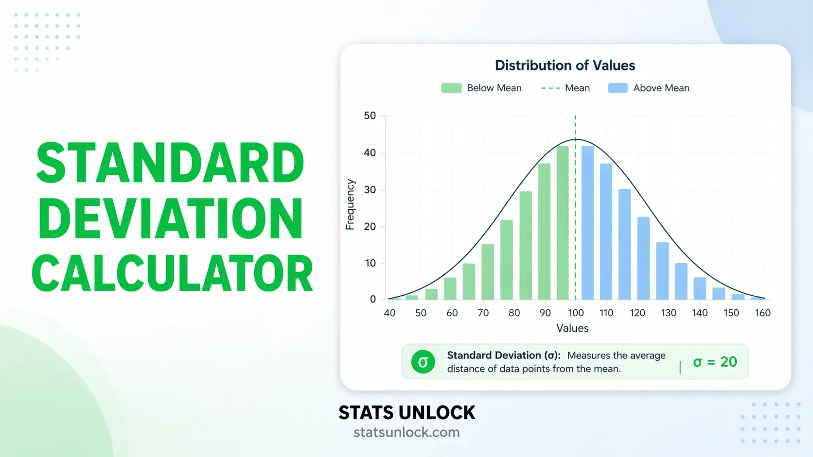
Standard Deviation Calculator with Steps | StatsUnlock

A standard deviation calculator finds how far values typically sit from their mean: subtract the mean from each value, square the gaps, add them, divide by n − 1 for a sample (or n for a population), then take the square root.

For the 16 values 52, 48, 55, 61, 47, 50, 58, 53, 49, 56, 51, 54, 46, 57, 50, 52 the mean is 52.4375, the sum of squares is 263.9375, the sample variance is 17.5958 and the sample standard deviation is 4.1947. The population standard deviation is 4.0615. A bigger SD means more spread. The SD is never negative, and it is zero only when every value is the same.

Rule of thumb: use the sample SD (n − 1, Excel STDEV.S) unless you measured every member of the group. For bell-shaped data about 68% of values lie within 1 SD of the mean, 95% within 2 SD and 99.7% within 3 SD. A coefficient of variation under 10% is low spread, 10% to 30% is moderate, and above 30% is high.

The standard deviation (SD) is the typical distance between each value and the mean of the data. It is measured in the same units as the data, so an SD of 4.19 mm means leaf lengths usually sit about 4 mm above or below their average. The variance is the same idea before the square root, so it is measured in squared units (mm²), which is harder to read.

What it actually measures: spread, also called dispersion or variability. Two groups can share the same mean of 52.5 and still be very different. In the sample dataset on this page, Site A has an SD of 4.19 mm while Site B has an SD of 8.05 mm, almost double, even though their means differ by only 0.13 mm. The mean tells you where the data sit. The SD tells you how tightly they sit there.

A worked one-liner: for 2, 4, 4, 4, 5, 5, 7, 9 the mean is 5, the squared deviations add to 32, so the population SD is √(32 ÷ 8) = 2 and the sample SD is √(32 ÷ 7) = 2.1381.

Who uses it: laboratories use the SD and the relative standard deviation to judge measurement precision. Teachers and psychologists use it to turn scores into z-scores. Manufacturers use it to set control limits at ±3 SD. Ecologists use it to compare how variable body size or yield is between sites. Finance uses it as a measure of risk, called volatility. Clinical trials report every baseline variable as mean ± SD.

4.1 What the standard deviation tells you

The standard deviation is the typical distance between a value and the mean. If exam scores have a mean of 66 and an SD of 5, a typical student scored about 5 points above or below 66. The SD is in the same units as your data, which is why it is the measure people quote. Its square, the variance, is in squared units and is mostly used inside other formulas.

A useful mental picture: the SD is roughly the radius of the cloud of data around its centre. A small SD means a tight cloud. A large SD means a loose one. It is not the average distance exactly (that is the mean absolute deviation, which is always a little smaller), because squaring gives extra weight to values far from the mean.

4.2 Is my standard deviation high or low?

There is no universal "good" standard deviation, because the SD depends on the units and the scale. An SD of 5 is tiny for incomes in dollars and enormous for blood potassium in mmol/L. Three questions settle it:

• Compared with the mean? Use the coefficient of variation. Under 10% is low spread, 10% to 30% moderate, above 30% high. Laboratory assays usually aim for a CV under 5%.
• Compared with the range of the scale? On a 1 to 5 Likert item the largest possible SD is about 2. An SD of 1.1 is moderate disagreement; above 1.5 means opinions are split.
• Compared with published values? Reference SDs exist for most clinical and educational measures. An SD far above the literature often points to a mixed sample or a data entry problem.

4.3 Sample SD (n − 1) versus population SD (n)

Dividing by n − 1 instead of n is called Bessel’s correction. When you work from a sample, the deviations are measured from the sample mean, which sits closer to the data than the true population mean does. That makes the sum of squares slightly too small. Dividing by n − 1 (the degrees of freedom) corrects the variance so it is unbiased on average.

For the worked example the two answers are 4.1947 and 4.0615, a difference of about 3%. With n = 100 the gap falls to 0.5%, and with n = 5 it is 12%. Use the population SD only when your data contain every member of the group you want to describe, such as all 30 students in one class when you have no wish to generalise beyond them.

4.4 The 68-95-99.7 rule and when it fails

For data that follow a normal (bell-shaped) distribution, about 68% of values lie within 1 SD of the mean, 95% within 2 SD (1.96 SD exactly) and 99.7% within 3 SD. The calculator counts how many of your values actually fall in each band. In the worked example the counts are 62.5%, 93.75% and 100%, close to the rule for only 16 values.

When the counts are far from the rule, the data are not bell shaped and you should not use the rule to make statements like "95% of patients lie between". Chebyshev’s inequality is the safe fallback: for any distribution at all, at least 75% of values lie within 2 SD and at least 88.9% within 3 SD.

4.5 How outliers inflate the standard deviation

Because every deviation is squared, one value far from the mean can dominate the SD. Chart 4 shows each value’s squared deviation. In the worked example the value 61 alone supplies 73.3 of the 263.9 total, or 27.8% of the sum of squares, even though it is just one value out of 16. In Example 3 below a single typing error makes the SD almost 14 times bigger.

Compare the ordinary SD with the robust SD (1.4826 × the median absolute deviation). If the ordinary SD is more than about 1.5 times the robust one, a few extreme values are driving it. Do not delete them blindly. Check the raw records, fix genuine errors, and report the robust measure alongside if real extremes remain.

4.6 The confidence interval for the standard deviation

Your SD is an estimate of the population SD, and like any estimate it has uncertainty. The calculator uses the chi-square distribution to build an interval: √[(n − 1)s² ÷ χ²_upper] to √[(n − 1)s² ÷ χ²_lower]. The interval is not symmetric around s, because the SD can never go below zero.

The width surprises most people. With n = 16 the 95% interval for the worked example runs from 3.10 to 6.49, so the true SD could plausibly be 25% lower or 55% higher than the estimate. With n = 6 the upper limit is nearly four times the lower one. This interval relies heavily on normality, much more than the interval for a mean, so treat it with care when the data are skewed.

4.7 Standard deviation versus standard error

This is the most common mix-up in published research. The SD describes how variable the individual values are. It does not shrink as you collect more data, it just becomes a better estimate. The standard error of the mean, SE = s ÷ √n, describes how precisely the mean has been estimated, and it does shrink as n grows.

Use mean ± SD to describe your sample, for example in Table 1 of a paper. Use SE, or better a confidence interval, when you want to show how well the mean is pinned down. Error bars of ±SE look about √n times shorter than ±SD bars, which is why some authors prefer them and why readers must always be told which one is shown. Chart 2 draws both so you can see the difference.

4.8 Comparing spread across groups

When you enter two or more groups, the calculator reports the pooled SD, the combined SD and the Brown-Forsythe test. The pooled SD averages the within-group variances weighted by their degrees of freedom. It is the SD used in Cohen’s d and in the classic Student t-test. The combined SD treats all values as one sample, so it also includes the differences between group means and is usually larger.

The Brown-Forsythe test asks whether the groups differ in spread. It runs an ANOVA on the distances from each group’s median, which makes it robust to non-normal data. A p-value below 0.05 means the spreads differ: report each SD separately and prefer Welch-type tests when you compare means. A ratio of largest to smallest SD above 2 is a common warning sign even when the test is not significant.

4.9 Coefficient of variation and relative standard deviation

The coefficient of variation (CV), also called the relative standard deviation (RSD), is the SD divided by the mean, times 100. It lets you compare spread between groups on different scales, such as the variability of body mass in mice and in elephants. A CV of 8% means the typical deviation is 8% of the mean.

The CV is only meaningful on a ratio scale with a true zero and a positive mean. Do not compute it for temperatures in Celsius, for z-scores, or for differences that can be negative. When the mean is near zero, the CV explodes and becomes useless.

4.10 Can the standard deviation be negative, or bigger than the mean?

The SD can never be negative, because it is a square root of a sum of squares. It is zero only when every value is identical. If software shows a negative SD, a formula has been typed wrongly.

The SD can be bigger than the mean. That is common and correct for data that are bounded at zero and skewed to the right, such as hospital stays, insurance claims or species counts. For such data, mean ± 2 SD gives a negative lower bound, which is impossible, so report the median and IQR as well. Example 4 below shows an SD of 10.60 with a mean of 6.16.

4.11 What the standard deviation cannot tell you

The SD says nothing about the shape of the data. A symmetric sample, a skewed sample and a sample with two separate clusters can all share an SD of 10. It also says nothing about why the data vary: measurement error, real biological differences and data entry mistakes all add to it in the same way. And on its own it is not a test. Two groups with different SDs may differ by chance, which is what the Brown-Forsythe test checks.

The SD of a biased sample is a precise answer to the wrong question. No formula fixes a sample that does not represent the population.

4.12 Practical judgement

Look at Chart 1 before you look at the number. Check that the data form one group, not two. Check the outlier flags and the robust SD. Decide between n − 1 and n before you report, and say which you used. Then report mean ± SD with n, add the median and IQR when the data are skewed, and give the confidence interval for σ when the SD itself is your result, for example in a reliability or quality control study.

When reporting standard deviation calculator results in APA format, give the mean, the SD and n together, say whether you used the sample or population formula, and match decimal places to your measurement. The five templates below fill in automatically after you press Calculate.

▶ Run the analysis above to auto-fill all five examples with your results.

5.1 Methods wording

"Continuous variables are presented as mean ± standard deviation (SD), calculated with the n − 1 denominator. Variables with marked skew are additionally summarised as median and interquartile range." One sentence like this, placed once, saves every later table from repeating it.

5.2 The Results sentence

Lead with the finding, then the numbers in brackets: "Leaf length on the south slope was considerably more variable than on the north slope (SD = 8.05 mm vs 4.19 mm; Brown-Forsythe F(1, 30) = 7.79, p = .009), although the means were almost identical (52.56 vs 52.44 mm)."

5.3 Tables and figures

• Use one column per group and rows for mean (SD), with n in the column header.
• Do not use the ± symbol in a table cell when the caption says "mean (SD)". Pick one format.
• Every error bar must be labelled in the caption: "Error bars show ±1 SD."
• Show the raw data points next to bars when n is under about 30, as Chart 1 does.

5.4 The Discussion sentence

Interpret the spread, not just the centre: "The larger SD on the south slope suggests more heterogeneous growing conditions, which may matter more for management than the near-identical mean." Spread is often the real biological or practical story.

5.5 Final reporting checklist

• Mean, SD and n given together for every group.
• Sample (n − 1) or population (n) formula stated.
• SD and SE never confused; error bars labelled.
• Outlier rule stated, and any removed values disclosed.
• Median and IQR added when skewness is above about 1, or when SD exceeds the mean for positive data.
• Confidence interval for σ given when the SD itself is a key result.

This flowchart shows how the standard deviation is calculated, step by step, from a raw column of numbers to a checked and reportable SD. Every box uses the same worked example as the Excel, R and Python sections: 16 leaf lengths in millimetres from Site A.

Check any box yourself: the Excel sheet in Section 9, the R script in Section 10 and the Python script in Section 11 all return a sum of squares of 263.9375, a sample SD of 4.1947 and a population SD of 4.0615 for this dataset.

1. Enter your data. Type or paste comma-separated numbers into the first box, in the format the placeholder shows: 52, 48, 55, 61, 47, .... Spaces, tabs and new lines also work.
2. Name each group. Click the group name above each box and type something meaningful, such as North slope. The name flows into the tables, charts and report sentences.
3. Add more groups to compare spread. Press Add group for each extra sample. With two or more groups you also get the pooled SD, the combined SD and the Brown-Forsythe test.
4. Or upload a CSV or Excel file. On the Upload tab choose your file, then click every column you want. Each clicked column becomes its own group, highlighted in the preview.
5. Or try a sample dataset. Ten built-in datasets cover clean data, skewed income, a Likert scale, a small sample and a dataset with a typing error.
6. Choose sample or population SD. Keep the default sample SD (n − 1) unless you measured every member of the population. Both are always shown in the table.
7. Set the confidence level and outlier fence. 95% and 1.5 × IQR are the usual choices.
8. Press Calculate Standard Deviation. Nothing is computed until you do. Changing any input clears old results, so you never read stale numbers.
9. Read the checks and the four charts. Look for outlier flags, strong skew and an SD driven by one value in Chart 4 before you trust the number.
10. Report and export. Copy a ready-made sentence from Section 5, then use Download Doc for a text report or Download PDF for a printable version with charts.

Excel has six standard deviation functions, and picking the wrong one is the single most common reason a spreadsheet answer disagrees with a paper or with R. The arithmetic itself is one formula. What trips people up is STDEV.S versus STDEV.P, blank cells and text that silently shrink n, and the confidence interval for the SD, which has no built-in function at all. This section walks through all of it with the spreadsheet shown at each step.

9.1 The functions you need

The Analysis ToolPak (File → Options → Add-ins → Manage Excel Add-ins → tick Analysis ToolPak) gives a Descriptive Statistics table under Data → Data Analysis. Its "Standard Deviation" row is the sample SD, the same as STDEV.S.

9.2 Step by step

9.3 The awkward cases

Standard deviation of a frequency table. Put class midpoints in A, frequencies in B, then:

For the frequency table in Section 2C (midpoints 42.5 to 67.5) this gives 6.1660. The classic mistake is dividing by the number of classes instead of the total frequency.

Standard deviation from a standard error. =SE*SQRT(n). A paper reporting SE = 0.35 with n = 49 implies SD = 2.45. Forgetting this step is the most common error in meta-analysis data extraction.

Ignoring zeros that mean "missing". =STDEV.S(IF(A2:A17<>0,A2:A17)) entered as an array formula (Ctrl + Shift + Enter in older Excel). Blank cells are ignored automatically, but zeros are counted.

9.4 Why your Excel answer might differ from R or Python

9.5 Charting mean ± SD in Excel

1. Select your group names and their means.
2. Insert → Charts → Clustered Column.
3. Click the chart, press the + button, tick Error Bars, then More Options → Custom → Specify Value and select the cells holding each group’s SD for both the positive and negative values.
4. Do not use Excel’s built-in "Standard Deviation" error bar option. It computes one SD across all the bar heights, not the SD of each group’s data, and it is wrong for this purpose.
5. Write in the caption "Error bars show ±1 SD". An unlabelled error bar cannot be interpreted.

Chart 2 in Section 3 of this page draws SD and SE error bars side by side automatically, which is a quick way to check your Excel chart.

9.6 Excel errors you will probably hit

R gives you the sample standard deviation in two letters, sd(x), but a bare SD is rarely all you need to report. The script below is complete and runnable. It shows every step of the calculation, adds the population SD, the standard error, the CV, a chi-square confidence interval for σ and two robust checks, prints a plain-English verdict, and saves one publication-ready figure at 300 dpi. It uses base R only, so there is nothing to install.

10.1 The complete script

R, base only, saves sd_plot.png

# ============================================================
# Standard deviation with steps, CI for sigma and one figure
# StatsUnlock - https://statsunlock.com/standard-deviation-calculator/
# Base R only. No packages to install.
# ============================================================

# ---- 1. Your data ------------------------------------------
# Replace with your own values, or read a CSV:
#   x <- read.csv("data.csv")$column_name
x <- c(52, 48, 55, 61, 47, 50, 58, 53,
       49, 56, 51, 54, 46, 57, 50, 52)
x <- x[!is.na(x)]                  # drop missing values first

label <- "Site A, north slope"
units <- "mm"
conf  <- 0.95

# ---- 2. The calculation, step by step ----------------------
n      <- length(x)
mean_x <- mean(x)
dev    <- x - mean_x               # deviations, they sum to 0
ss     <- sum(dev^2)               # sum of squares (Excel DEVSQ)
var_s  <- ss / (n - 1)             # sample variance, same as var(x)
sd_s   <- sqrt(var_s)              # sample SD, same as sd(x)
var_p  <- ss / n                   # population variance
sd_p   <- sqrt(var_p)              # population SD
se     <- sd_s / sqrt(n)
cv     <- sd_s / abs(mean_x) * 100

# ---- 3. Confidence interval for sigma (chi-square) ---------
a     <- 1 - conf
ci_lo <- sqrt(ss / qchisq(1 - a / 2, df = n - 1))
ci_hi <- sqrt(ss / qchisq(a / 2,     df = n - 1))

# ---- 4. Robust checks ---------------------------------------
mad_robust <- mad(x)               # 1.4826 x median absolute deviation
iqr_sd     <- IQR(x) / 1.349
within2    <- mean(abs(dev) <= 2 * sd_s) * 100

cat(sprintf("n                  = %d\n", n))
cat(sprintf("mean               = %.4f\n", mean_x))
cat(sprintf("sum of squares     = %.4f\n", ss))
cat(sprintf("sample variance    = %.4f\n", var_s))
cat(sprintf("sample SD (n-1)    = %.4f\n", sd_s))
cat(sprintf("population SD (n)  = %.4f\n", sd_p))
cat(sprintf("standard error     = %.4f\n", se))
cat(sprintf("CV                 = %.2f%%\n", cv))
cat(sprintf("%d%% CI for sigma   = %.4f to %.4f\n", round(conf * 100), ci_lo, ci_hi))
cat(sprintf("robust SD (MAD)    = %.4f   IQR/1.349 = %.4f\n", mad_robust, iqr_sd))
cat(sprintf("within 2 SD        = %.1f%%\n", within2))
cat(sprintf("Verdict: SD = %.2f %s, CV = %.1f%% -> %s spread%s\n", sd_s, units, cv,
    if (cv < 10) "low" else if (cv <= 30) "moderate" else "high",
    if (sd_s / mad_robust > 1.5) ", but outliers may be inflating it" else ""))

# ---- 5. One figure, two panels -----------------------------
png("sd_plot.png", width = 3000, height = 1500, res = 300)
par(mfrow = c(1, 2), mar = c(4.5, 4.5, 3.5, 1), family = "sans")

# left: every value with mean +/- 1 and 2 SD bands
set.seed(42)                       # reproducible jitter
jit <- runif(n, -0.25, 0.25)
plot(jit, x, xlim = c(-0.6, 0.6), xaxt = "n", xlab = "", ylab = units,
     pch = 21, bg = adjustcolor("#16a34a", 0.75), col = "white", cex = 1.6,
     ylim = range(c(x, mean_x + c(-2, 2) * sd_s)), las = 1,
     main = sprintf("%s\nmean = %.2f, SD = %.2f", label, mean_x, sd_s), cex.main = 0.95)
rect(-0.4, mean_x - 2 * sd_s, 0.4, mean_x + 2 * sd_s, col = adjustcolor("#16a34a", 0.08), border = NA)
rect(-0.4, mean_x - sd_s,     0.4, mean_x + sd_s,     col = adjustcolor("#16a34a", 0.18), border = NA)
segments(-0.4, mean_x, 0.4, mean_x, lwd = 3, col = "#15803d")
points(jit, x, pch = 21, bg = adjustcolor("#16a34a", 0.75), col = "white", cex = 1.6)

# right: histogram with normal curve and SD lines
h <- hist(x, breaks = "Sturges", plot = FALSE)
plot(h, col = "#e9d5ff", border = "#9333ea", main = "Histogram with +/- 1, 2, 3 SD",
     xlab = sprintf("Value (%s)", units), las = 1, cex.main = 0.95,
     xlim = mean_x + c(-3.3, 3.3) * sd_s)
bw <- diff(h$breaks)[1]
curve(n * bw * dnorm(x, mean_x, sd_s), add = TRUE, col = "#ea580c", lwd = 2.4)
abline(v = mean_x + (-3:3) * sd_s, lty = c(3, 2, 2, 1, 2, 2, 3),
       col = c("#b91c1c", "#ca8a04", "#0f766e", "#111827", "#0f766e", "#ca8a04", "#b91c1c"))

dev.off()
cat("\nSaved sd_plot.png\n")

Run it with Rscript sd_script.R from a terminal, or paste it into the RStudio console. It prints n = 16, sample SD = 4.1947, population SD = 4.0615 and a 95% CI for sigma of 3.0987 to 6.4922.

10.2 What each part does

10.3 What the figure shows

The left panel plots every value with a little horizontal jitter. The dark green band is the mean ± 1 SD and the pale band is ± 2 SD, with the mean as a thick line. You can see at a glance that most points sit inside the dark band and none sit outside the pale one. The right panel is a histogram with a normal curve of the same mean and SD drawn over it, plus lines at ±1, 2 and 3 SD. If the bars roughly follow the curve, mean ± SD is a fair summary.

10.4 Common R problems and fixes

10.5 Useful one-liners

Python has at least four ways to get a standard deviation, and they do not agree by default. NumPy’s np.std() returns the population SD unless you pass ddof=1, while pandas and the statistics module return the sample SD. The script below sets ddof explicitly, prints every step, adds a chi-square confidence interval for σ and saves one 300 dpi figure.

Install with pip install numpy scipy matplotlib if you do not already have them.

11.1 The complete script

Python 3, saves sd_plot.png

# ============================================================
# Standard deviation with steps, CI for sigma and one figure
# StatsUnlock - https://statsunlock.com/standard-deviation-calculator/
# ============================================================

import numpy as np
import matplotlib
matplotlib.use("Agg")              # save to file without opening a window
import matplotlib.pyplot as plt
from scipy import stats

# ---- 1. Your data ------------------------------------------
# Replace this list with your own values, or read a CSV:
#   import pandas as pd
#   x = pd.read_csv("data.csv")["column_name"].to_numpy(dtype=float)
x = np.array([52, 48, 55, 61, 47, 50, 58, 53,
              49, 56, 51, 54, 46, 57, 50, 52], dtype=float)
x = x[~np.isnan(x)]                # drop missing values first

label, units, conf = "Site A, north slope", "mm", 0.95

# ---- 2. The calculation, step by step ----------------------
n = x.size
mean_x = x.mean()
dev = x - mean_x                   # deviations, they sum to 0
ss = np.sum(dev ** 2)              # sum of squares (Excel DEVSQ)
sd_s = np.std(x, ddof=1)           # sample SD, matches STDEV.S and R sd()
sd_p = np.std(x, ddof=0)           # population SD, NumPy default
var_s = sd_s ** 2
se = sd_s / np.sqrt(n)
cv = sd_s / abs(mean_x) * 100

# ---- 3. Confidence interval for sigma (chi-square) ---------
a = 1 - conf
ci_lo = np.sqrt(ss / stats.chi2.ppf(1 - a / 2, n - 1))
ci_hi = np.sqrt(ss / stats.chi2.ppf(a / 2, n - 1))

# ---- 4. Robust checks ---------------------------------------
mad_robust = stats.median_abs_deviation(x, scale="normal")   # 1.4826 x MAD
q1, q3 = np.percentile(x, [25, 75])
iqr_sd = (q3 - q1) / 1.349
within2 = np.mean(np.abs(dev) <= 2 * sd_s) * 100

print(f"n                  = {n}")
print(f"mean               = {mean_x:.4f}")
print(f"sum of squares     = {ss:.4f}")
print(f"sample variance    = {var_s:.4f}")
print(f"sample SD (n-1)    = {sd_s:.4f}")
print(f"population SD (n)  = {sd_p:.4f}")
print(f"standard error     = {se:.4f}")
print(f"CV                 = {cv:.2f}%")
print(f"{conf:.0%} CI for sigma   = {ci_lo:.4f} to {ci_hi:.4f}")
print(f"robust SD (MAD)    = {mad_robust:.4f}   IQR/1.349 = {iqr_sd:.4f}")
print(f"within 2 SD        = {within2:.1f}%")
level = "low" if cv < 10 else "moderate" if cv <= 30 else "high"
flag = ", but outliers may be inflating it" if sd_s / mad_robust > 1.5 else ""
print(f"Verdict: SD = {sd_s:.2f} {units}, CV = {cv:.1f}% -> {level} spread{flag}")

# ---- 5. One figure, two panels -----------------------------
rng = np.random.default_rng(42)    # reproducible jitter
fig, (ax1, ax2) = plt.subplots(1, 2, figsize=(10, 5))

jit = rng.uniform(-0.25, 0.25, n)
ax1.axhspan(mean_x - 2 * sd_s, mean_x + 2 * sd_s, xmin=0.15, xmax=0.85, color="#16a34a", alpha=0.08)
ax1.axhspan(mean_x - sd_s, mean_x + sd_s, xmin=0.15, xmax=0.85, color="#16a34a", alpha=0.18)
ax1.hlines(mean_x, -0.4, 0.4, color="#15803d", lw=3)
ax1.scatter(jit, x, s=70, color="#16a34a", alpha=0.8, edgecolor="white")
ax1.set_xlim(-0.6, 0.6); ax1.set_xticks([]); ax1.set_ylabel(units)
ax1.set_title(f"{label}\nmean = {mean_x:.2f}, SD = {sd_s:.2f}", fontsize=10)

counts, edges, _ = ax2.hist(x, bins="sturges", color="#e9d5ff", edgecolor="#9333ea")
grid = np.linspace(mean_x - 3.3 * sd_s, mean_x + 3.3 * sd_s, 200)
ax2.plot(grid, n * (edges[1] - edges[0]) * stats.norm.pdf(grid, mean_x, sd_s), color="#ea580c", lw=2.4)
for k, c in zip(range(-3, 4), ["#b91c1c", "#ca8a04", "#0f766e", "#111827", "#0f766e", "#ca8a04", "#b91c1c"]):
    ax2.axvline(mean_x + k * sd_s, color=c, ls="-" if k == 0 else "--", lw=1.4)
ax2.set_title("Histogram with +/- 1, 2, 3 SD", fontsize=10)
ax2.set_xlabel(f"Value ({units})")

fig.tight_layout()
fig.savefig("sd_plot.png", dpi=300, bbox_inches="tight")
print("\nSaved sd_plot.png")

Run it with python sd_script.py. It prints n = 16, mean = 52.4375, sum of squares = 263.9375, sample SD = 4.1947, population SD = 4.0615 and a 95% CI for sigma of 3.0987 to 6.4922, matching Excel and R exactly.

11.2 What each part does

11.3 What the figure shows

The two panels match the R figure exactly: every value with mean ± 1 and 2 SD bands on the left, and the histogram with a fitted normal curve and SD lines on the right. Same data, same seed, same picture, which is a quick visual proof that the two scripts agree.

11.4 Common Python problems and fixes

11.5 Useful one-liners

Run the script with python sd_script.py from a terminal. In Jupyter, remove the matplotlib.use("Agg") line and add plt.show() at the end to see the figure inline.

12.1 Which standard deviation should you use?

What to conclude: the n − 1 sample SD is the default. Switch only when the situation in the left column clearly applies.

12.2 Empirical rule versus Chebyshev’s inequality

What to conclude: only use the 68-95-99.7 rule when your data look bell shaped. Otherwise quote the Chebyshev minimum, which holds for every distribution (Pukelsheim, 1994).

12.3 How precise is a standard deviation? 95% CI as a multiple of s

What to conclude: you need about 30 values before the SD is known to within roughly 20% to 35%, and about 100 to get within 15%. Multiply your own s by these factors for a quick interval (normal data assumed).

12.4 Chi-square critical values for the CI of σ

What to conclude: for a 95% interval divide (n − 1)s² by the 0.975 value for the lower limit and by the 0.025 value for the upper limit, then take square roots. The worked example uses df = 15.

12.5 Bessel correction and the c4 constant

What to conclude: n − 1 makes the variance unbiased, but the SD itself is still slightly too small on average. Dividing s by c4 removes that bias, which matters in quality control charts with small subgroups.

12.6 Turning other spread measures into an SD

What to conclude: SE and CI conversions are exact; the others are estimates that assume a bell-shaped distribution (Wan et al., 2014; Hozo et al., 2005). The Summary tab in Section 2 does all of these for you.

12.7 Coefficient of variation bands

What to conclude: these bands are conventions, not laws. Always compare a CV with values published for the same measurement in your field.

Study design: the standard deviation assumes independent measurements of one quantity on an interval or ratio scale, taken the same way for every unit, so that differences between values reflect real variation plus ordinary measurement error.

1. Define the unit of observation before you calculate standard deviation. Decide whether one value is one plant, one patient or one repeat reading. Mixing repeat readings with separate subjects shrinks the SD and makes the data look more consistent than they are.
2. Choose sample or population SD at the design stage. If you will generalise beyond the units you measure, plan to use the sample standard deviation (n − 1) and say so in the protocol.
3. Plan enough observations for a stable SD. Aim for at least 20 to 30 per group. With 10 values the 95% interval for σ still spans a factor of 2.65 (Table 12.3).
4. Randomise selection. A convenience sample often has less spread than the population, because people or sites that are easy to reach tend to be similar.
5. Fix the instrument, units and resolution. Switching instruments or observers mid-study adds variation that has nothing to do with the subject.
6. Record missing values as blank, never as zero. A fake zero is usually far from the mean and can double the standard deviation on its own.
7. Write the outlier rule in advance. State that values beyond 1.5 × IQR from the quartiles will be checked against raw records and corrected only if they are errors.
8. Keep groups in separate columns or label them clearly. Mixing two populations inflates the standard deviation and hides a two-peaked distribution.
9. Enter data twice or verify a random 10%. Example 3 shows how one typing error can make the SD almost 14 times larger.
10. Check standard deviation calculation results in two tools. Run the same column through this page and Excel or R. Agreement to four decimals confirms the right formula and range.

Long format like this pastes straight into R or pandas. For this calculator, put each group in its own column (wide format) and click the columns on the Upload tab.

Minimum sample: two values give a sample SD, but treat anything under 10 per group as a rough guide and always report the confidence interval for σ. Pre-registration line: "Dispersion will be summarised as the sample SD (n − 1) with a 95% chi-square confidence interval; outliers will be screened with Tukey fences at 1.5 × IQR." Common mistakes: pooling repeat readings as if they were separate subjects, typing 0 for missing values, mixing units within a column, and reporting SE while calling it SD.

This free standard deviation calculator is designed for students checking homework, researchers describing a sample, teachers building z-scores and analysts who need the SD, variance and CV for one or many groups with the working shown.

Four real-world examples

• Clinical baseline table: age, weight and blood pressure reported as mean ± SD per treatment arm.
• Laboratory precision: the SD and CV of 10 replicate assays judge whether a method is repeatable.
• Education: exam SDs show whether a new teaching method helps everyone equally or widens the gap.
• Field ecology: the SD of body size or yield between sites reveals how patchy a habitat is.

Study design guidance

Plan the sample size around the precision you need for the SD itself, not just for the mean (Table 12.3). When the SD will feed into a power calculation for a later study, use the upper confidence limit of σ rather than the point estimate, so the next study is not underpowered.

Decision tree: the right tool for your question

Assumptions

1. Independent observations. Each value comes from a different unit. Check: the design; no repeat readings counted as separate subjects. If it fails: the SD is biased downward, because repeats are more alike than separate units.
2. Interval or ratio scale. Differences between values mean the same thing everywhere on the scale. Check: the measurement type. If it fails: on ordinal scales the SD has no clean meaning and can over or under state disagreement.
3. One population per group. Check: Chart 1 and Chart 3 for two separate clusters. If it fails: the SD is biased upward, since the gap between the clusters is counted as spread.
4. Roughly normal data for the 68-95-99.7 rule and the CI for σ. Check: skewness, the empirical rule counts and Chart 3. If it fails: the CI for σ is too narrow with heavy tails, and the rule misstates coverage.
5. Correct values. Check: outlier flags and the ratio of ordinary to robust SD. If it fails: recording errors bias the SD upward, often strongly.

Limitations

1. The SD is not robust: one extreme value can dominate it. Alternative: median absolute deviation or IQR, both reported above.
2. The SD says nothing about shape. Alternative: the five number summary and a box plot.
3. The CI for σ relies heavily on normality. Alternative: a bootstrap interval in R or Python for skewed data.
4. Grouped-data SDs are approximations. Alternative: obtain the raw values where possible.
5. SD from IQR or range assumes normal data. Alternative: ask authors for the SD, or use the methods of Wan et al. (2014) with care.
6. The Brown-Forsythe test has low power with small groups. Alternative: report the SD ratio and confidence intervals for each σ.

A standard deviation calculator turns a column of numbers into one figure that describes how tightly they cluster around their mean. The arithmetic is short: find the mean, square each distance from it, add those squares, divide by n − 1 and take the square root. For the worked example that gives 4.1947 mm. What makes the number useful, or misleading, is everything around that arithmetic.

The first decision is sample versus population. Almost all research data are samples, so the n − 1 formula and Excel’s STDEV.S are the right default. The second is whether the SD can be trusted at all. One typing error, a zero used for a missing value, or two populations mixed into one column can inflate it many times over, which is why this page shows every value, flags outliers and reports a robust SD beside the ordinary one.

The third is how precise the SD is. A standard deviation from 16 values could easily be 25% too high or 55% too low, and from 6 values the uncertainty is far larger. When the SD itself matters, for a reliability study or for planning sample size, report its confidence interval. And never confuse it with the standard error: SD describes the people or plants, SE describes the mean.

Finally, report it properly: mean ± SD with n, the formula you used, and the median and IQR when the data are skewed. Paste your data into this standard deviation calculator, read the checks before the headline number, and copy a ready-made sentence from Section 5.

These peer-reviewed sources support the methods used in this standard deviation calculator: the sample and population formulas, stable computation, confidence intervals, robust alternatives, pooled and grouped SDs, and best practice in reporting spread.

1. Altman, D. G., & Bland, J. M. (2005). Standard deviations and standard errors. BMJ, 331(7521), 903. https://doi.org/10.1136/bmj.331.7521.903
2. Bland, J. M., & Altman, D. G. (1996). Statistics notes: Measurement error. BMJ, 312(7047), 1654. https://doi.org/10.1136/bmj.312.7047.1654
3. Brown, M. B., & Forsythe, A. B. (1974). Robust tests for the equality of variances. Journal of the American Statistical Association, 69(346), 364–367. https://doi.org/10.1080/01621459.1974.10482955
4. Chan, T. F., Golub, G. H., & LeVeque, R. J. (1983). Algorithms for computing the sample variance: Analysis and recommendations. The American Statistician, 37(3), 242–247. https://doi.org/10.1080/00031305.1983.10483115
5. Conover, W. J., Johnson, M. E., & Johnson, M. M. (1981). A comparative study of tests for homogeneity of variances, with applications to the outer continental shelf bidding data. Technometrics, 23(4), 351–361. https://doi.org/10.1080/00401706.1981.10487680
6. Cumming, G., Fidler, F., & Vaux, D. L. (2007). Error bars in experimental biology. Journal of Cell Biology, 177(1), 7–11. https://doi.org/10.1083/jcb.200611141
7. Hozo, S. P., Djulbegovic, B., & Hozo, I. (2005). Estimating the mean and variance from the median, range, and the size of a sample. BMC Medical Research Methodology, 5, 13. https://doi.org/10.1186/1471-2288-5-13
8. Hyndman, R. J., & Fan, Y. (1996). Sample quantiles in statistical packages. The American Statistician, 50(4), 361–365. https://doi.org/10.1080/00031305.1996.10473566
9. Lakens, D. (2013). Calculating and reporting effect sizes to facilitate cumulative science: A practical primer for t-tests and ANOVAs. Frontiers in Psychology, 4, 863. https://doi.org/10.3389/fpsyg.2013.00863
10. Lang, T. A., & Altman, D. G. (2015). Basic statistical reporting for articles published in biomedical journals: The "Statistical Analyses and Methods in the Published Literature" or the SAMPL Guidelines. International Journal of Nursing Studies, 52(1), 5–9. https://doi.org/10.1016/j.ijnurstu.2014.09.006
11. Leys, C., Ley, C., Klein, O., Bernard, P., & Licata, L. (2013). Detecting outliers: Do not use standard deviation around the mean, use absolute deviation around the median. Journal of Experimental Social Psychology, 49(4), 764–766. https://doi.org/10.1016/j.jesp.2013.03.013
12. Nagele, P. (2003). Misuse of standard error of the mean (SEM) when reporting variability of a sample. A critical evaluation of four anaesthesia journals. British Journal of Anaesthesia, 90(4), 514–516. https://doi.org/10.1093/bja/aeg087
13. Pukelsheim, F. (1994). The three sigma rule. The American Statistician, 48(2), 88–91. https://doi.org/10.1080/00031305.1994.10476030
14. Reed, G. F., Lynn, F., & Meade, B. D. (2002). Use of coefficient of variation in assessing variability of quantitative assays. Clinical and Diagnostic Laboratory Immunology, 9(6), 1235–1239. https://doi.org/10.1128/CDLI.9.6.1235-1239.2002
15. Rousseeuw, P. J., & Croux, C. (1993). Alternatives to the median absolute deviation. Journal of the American Statistical Association, 88(424), 1273–1283. https://doi.org/10.1080/01621459.1993.10476408
16. Sheppard, W. F. (1897). On the calculation of the most probable values of frequency-constants, for data arranged according to equidistant division of a scale. Proceedings of the London Mathematical Society, s1-29(1), 353–380. https://doi.org/10.1112/plms/s1-29.1.353
17. Sullivan, G. M., & Artino, A. R. (2013). Analyzing and interpreting data from Likert-type scales. Journal of Graduate Medical Education, 5(4), 541–542. https://doi.org/10.4300/JGME-5-4-18
18. Wan, X., Wang, W., Liu, J., & Tong, T. (2014). Estimating the sample mean and standard deviation from the sample size, median, range and/or interquartile range. BMC Medical Research Methodology, 14, 135. https://doi.org/10.1186/1471-2288-14-135
19. Weissgerber, T. L., Milic, N. M., Winham, S. J., & Garovic, V. D. (2015). Beyond bar and line graphs: Time for a new data presentation paradigm. PLoS Biology, 13(4), e1002128. https://doi.org/10.1371/journal.pbio.1002128
20. Welford, B. P. (1962). Note on a method for calculating corrected sums of squares and products. Technometrics, 4(3), 419–420. https://doi.org/10.1080/00401706.1962.10490022