Berger-Parker Dominance Index Calculator
Free online tool to compute the Berger-Parker dominance index (d) for ecology and biodiversity research — instant calculation, four colourful visualisations, full interpretation, and publication-ready report.
📥 Data Input
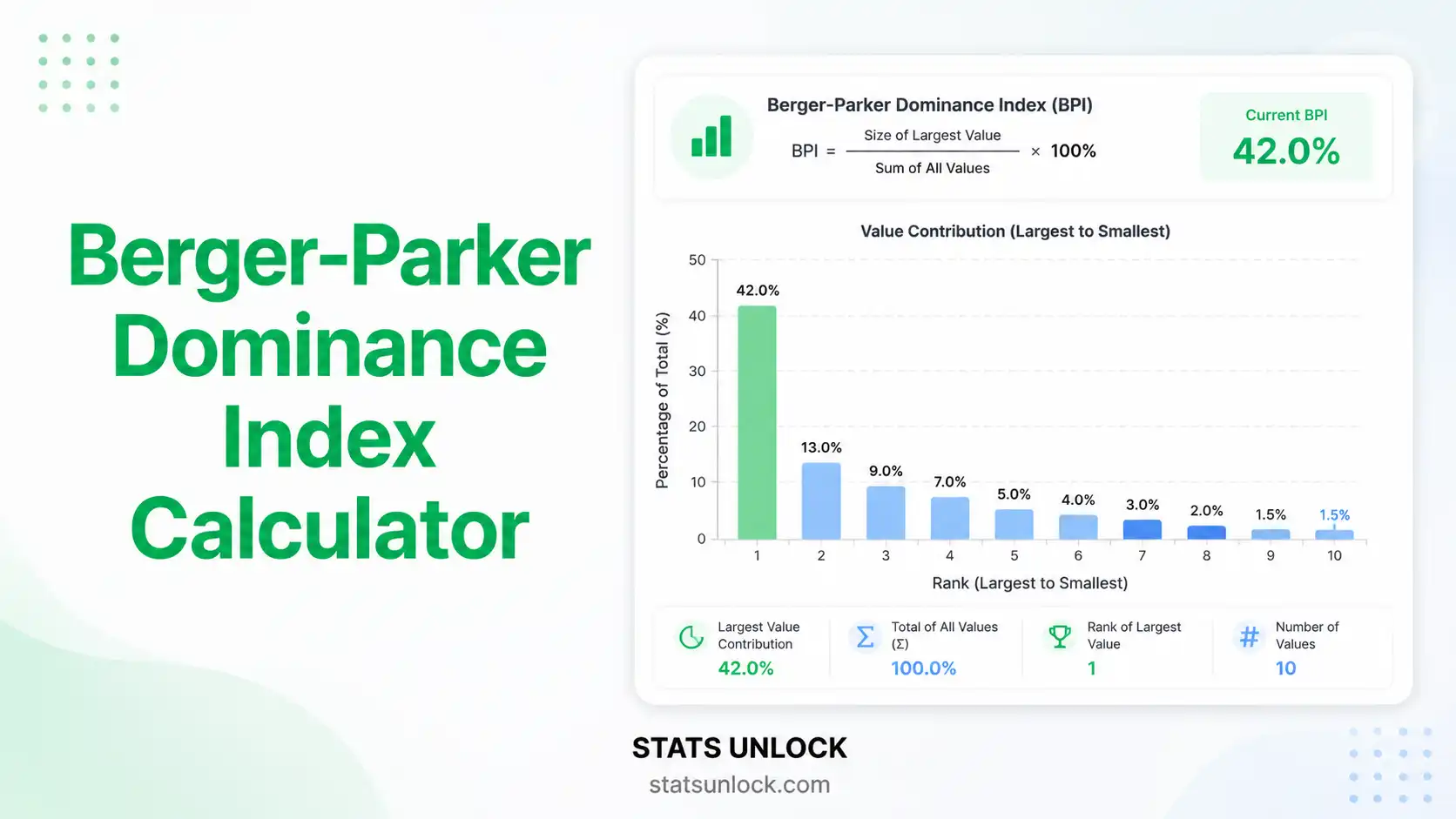
Enter species count data. The Berger-Parker index uses the most abundant species count divided by the total — d = Nmax / N.
0 valid values entered
Supports .csv, .txt, .xlsx, .xls. Select ONE column containing your species count values — each row in that column becomes one species/group.
Edit species and counts directly. Click "Add Species" to append more rows.
0 values entered
⚙️ Analysis Configuration
Used in interpretation, reporting examples, and the research poster.
Label for the taxonomic or functional group analysed.
Compare result against a published d value.
📊 Results Summary
Berger-Parker Dominance Index Equation
The formula for the Berger-Parker dominance index (d) is:
- d: Berger-Parker dominance index, ranging from near 0 (no dominance) to 1 (single-species dominance)
- Nmax: Number of individuals of the single most abundant species in the community
- N: Total number of individuals across all species
- 1/d: Berger-Parker reciprocal — the effective number of "equally common" dominant species
- Threshold: d > 0.5 indicates strong dominance by a single species; d < 0.3 indicates an even community
| Statistic | Value | Description |
|---|
📈 Four Visualisations
📖 Detailed Interpretation Results
✍️ How to Write Your Results in Research
Five fully detailed reporting templates auto-filled with your computed values. Copy the one that matches your audience.
🪧 Research Poster Panel
🔗 Related Biodiversity Calculators
The Berger-Parker index measures dominance — but a complete community profile usually pairs it with one or more complementary metrics. Use the calculators below to compute Shannon-Wiener diversity, Simpson's diversity, species richness, and evenness on the same dataset:
🧭 When to Use the Berger-Parker Dominance Index
Use it when:
- ✓ You need a quick, intuitive single-number summary of dominance
- ✓ Your study question is "how skewed is this community toward one species?"
- ✓ You have full counts of the most abundant species (it does not require complete enumeration of rare species)
- ✓ You are comparing dominance patterns across replicate sites with standardised effort
- ✓ You want a metric that is robust to small samples and easy to communicate to non-specialists
Avoid (or pair with another metric) when:
- ✗ Rare-species composition matters — Shannon-Wiener H' or Hill q=1 is more sensitive
- ✗ You need an evenness-only metric — use Pielou's J' or Simpson's E
- ✗ Sampling effort differs across sites — apply rarefaction first
- ✗ The community has multiple co-dominant species — Simpson's D captures this better
Real-world examples:
- 🦜 Pre/post-disturbance bird survey across a managed forest gradient
- 🦌 National park camera-trap mammal community structure (e.g. Yellowstone northern range)
- 🌳 Tree-species dominance in temperate or boreal forest plots
- 🐠 Reef fish community on impacted vs reference reefs
📘 How to Use This Tool — Step-by-Step Guide
- Enter your data: Paste comma-separated species counts in the textarea (e.g.,
52, 48, 55, 61, 47), upload a CSV/Excel file, or use the manual table. - Choose a sample dataset (optional): Five preloaded ecological datasets demonstrate different dominance regimes — from highly dominated logged-forest fragments to evenly distributed wetland communities.
- Configure the analysis: Add a Study Area name, edit the Group Name (default: "Bird Species"), choose decimal precision, and optionally enter a benchmark d value for comparison.
- Run the analysis: Click "Run Berger-Parker Analysis." Nothing runs automatically — you control when calculations happen.
- Read the summary cards: Green = low dominance / high evenness, amber = moderate dominance, red = high dominance (one species swamps the assemblage).
- Inspect the results table: See d, 1/d (reciprocal), Nmax, N, S (richness), dominant species name, and a moderate evenness comparison.
- Examine all four visualisations: Bar chart, pie chart, rank-abundance Whittaker plot, and a dominance threshold gauge — each reveals a different facet of community structure.
- Read the interpretation: Five paragraphs translate d into plain ecological language for park managers, funders, and journal reviewers.
- Copy a reporting example: Choose the journal, thesis, plain-language, abstract, monitoring, or research-poster style — each is auto-filled with your numbers.
- Export your results: Download the .txt Doc for fast sharing, or the PDF for printing and inclusion in field reports.
❓ Frequently Asked Questions
Q1. What is the Berger-Parker dominance index and when should I use it?
The Berger-Parker dominance index (d) is a simple biodiversity metric defined as the proportional abundance of the single most common species: d = Nmax / N. Values approach 0 in evenly distributed communities and approach 1 when one species swamps the assemblage. Use it when you want a quick, intuitive summary of dominance — for example, in pre/post-disturbance bird point counts, camera-trap mammal surveys, or tree-plot vegetation studies.
Q2. What data do I need to calculate the Berger-Parker index?
You only need a list of species counts (the number of individuals or detections per species). The index uses just Nmax (the largest count) and N (the sum of all counts), so it works with as little as two species. Standardised sampling effort across compared sites is essential. The Paste/Type, CSV/Excel upload, and Manual Table tabs all accept the same data — pick whichever fits your file.
Q3. What does a high vs low Berger-Parker value mean ecologically?
d > 0.5 means one species accounts for more than half of all individuals — strong dominance, often associated with disturbed or stressed habitat. d between 0.3 and 0.5 indicates moderate dominance — a typical structure for many natural communities. d < 0.3 indicates an even assemblage with no overwhelming dominant — characteristic of intact tropical forests and well-functioning wetlands. Always interpret in the context of habitat type and sampling effort.
Q4. How does Berger-Parker differ from Simpson's dominance?
Berger-Parker considers only the single most abundant species, while Simpson's D = Σpᵢ² sums squared proportions across all species. Berger-Parker is simpler and more intuitive but discards information about the rest of the abundance distribution. If two communities both have d = 0.4 but one is otherwise even and the other has a second sub-dominant taking 30%, Simpson's will distinguish them; Berger-Parker will not. Best practice: report both.
Q5. What are the assumptions and limitations of the Berger-Parker index?
The metric assumes (1) complete enumeration of the dominant species, (2) equal detection probability across taxa, and (3) standardised sampling effort. It is insensitive to rare species and to changes anywhere except in the dominant. For violated assumptions, pair with rarefaction (unequal effort) or with occupancy / N-mixture models (imperfect detection). Always pair with a richness metric such as S or Margalef's Dmg for context.
Q6. How much sampling effort do I need for a reliable d?
Practical minima: ≥ 30–50 individuals total for a stable estimate; ≥ 1000 trap nights for camera-trap mammal communities; ≥ 3 replicate plots/transects/stations for site-level inference. Always inspect a species accumulation curve to confirm that further sampling would not change which species is dominant. Small samples are mathematically computable but unreliable.
Q7. Can I compare d values between sites or seasons?
Yes — but only when sampling effort, methods, and taxonomic resolution are standardised. If effort differs, apply rarefaction or bootstrap resampling first. Mixing detection methods (e.g., point counts vs mist nets) will bias d. For formal comparison, use permutation tests on bootstrap resamples of d, or use the framework of Hill numbers (Chao & Jost, 2012) for unified diversity comparison.
Q8. How do I report the Berger-Parker index in an ecology journal?
Report d to 2 decimal places, the dominant species name, and pair with S (species richness), N (total individuals), and at least one additional metric (Shannon-Wiener H' or Pielou's J'). Example: "Community dominance was moderate (d = 0.34, S = 28, N = 412), with the Red-eyed Vireo as the single most abundant species; this paired with H' = 2.74 indicates an evenly distributed assemblage." See the five reporting examples in this tool for full templates.
Q9. Can I use this calculator for published research or a university thesis?
Yes, for educational use, exploratory analysis, and most undergraduate / postgraduate coursework. For peer-reviewed publication, verify the result against the R vegan package (diversity(), specnumber()) or PRIMER-E. Cite this tool as: StatsUnlock. (2025). Berger-Parker dominance index calculator. https://statsunlock.com/tools/berger-parker-dominance-index-calculator
Q10. My d value seems unexpectedly high or low — what might have gone wrong?
Common causes: (1) one outlier species with inflated counts (data entry typo), (2) wrong column selected from the uploaded spreadsheet, (3) under-detection of rare species inflating relative dominance, (4) unequal sampling effort across sites, or (5) accidental inclusion of non-target taxa (juveniles double-counted, observer error). Try loading the "Chesapeake Bay Wetland Point Count" sample dataset to confirm the tool computes correctly, then re-check your raw counts.
🏁 Detailed Conclusion
📚 References
The following references support the ecological methods used in this Berger-Parker dominance index calculator, covering biodiversity measurement, species abundance distributions, and best practices in ecological sampling.
- Berger, W. H., & Parker, F. L. (1970). Diversity of planktonic foraminifera in deep-sea sediments. Science, 168(3937), 1345–1347. https://doi.org/10.1126/science.168.3937.1345
- Magurran, A. E. (2004). Measuring biological diversity. Blackwell Publishing. Publisher page
- Magurran, A. E., & McGill, B. J. (Eds.). (2011). Biological diversity: Frontiers in measurement and assessment. Oxford University Press. Publisher page
- May, R. M. (1975). Patterns of species abundance and diversity. In M. L. Cody & J. M. Diamond (Eds.), Ecology and evolution of communities (pp. 81–120). Harvard University Press.
- Krebs, C. J. (1999). Ecological methodology (2nd ed.). Benjamin Cummings.
- Simpson, E. H. (1949). Measurement of diversity. Nature, 163, 688. https://doi.org/10.1038/163688a0
- Shannon, C. E., & Weaver, W. (1949). The mathematical theory of communication. University of Illinois Press.
- Hill, M. O. (1973). Diversity and evenness: A unifying notation and its consequences. Ecology, 54(2), 427–432. https://doi.org/10.2307/1934352
- Jost, L. (2006). Entropy and diversity. Oikos, 113(2), 363–375. https://doi.org/10.1111/j.2006.0030-1299.14714.x
- Chao, A., & Jost, L. (2012). Coverage-based rarefaction and extrapolation: Standardizing samples by completeness rather than size. Ecology, 93(12), 2533–2547. https://doi.org/10.1890/11-1952.1
- Oksanen, J., Simpson, G. L., Blanchet, F. G., et al. (2024). vegan: Community ecology package. R package version 2.6-6. https://CRAN.R-project.org/package=vegan
- Gotelli, N. J., & Colwell, R. K. (2001). Quantifying biodiversity: Procedures and pitfalls in the measurement and comparison of species richness. Ecology Letters, 4(4), 379–391. https://doi.org/10.1046/j.1461-0248.2001.00230.x
- Caruso, T., Pigino, G., Bernini, F., et al. (2007). The Berger-Parker index as an effective tool for monitoring the biodiversity of disturbed soils. Biodiversity and Conservation, 16(11), 3277–3285. https://doi.org/10.1007/s10531-006-9137-3
- Pielou, E. C. (1966). The measurement of diversity in different types of biological collections. Journal of Theoretical Biology, 13, 131–144. https://doi.org/10.1016/0022-5193(66)90013-0
- R Core Team. (2024). R: A language and environment for statistical computing. R Foundation for Statistical Computing. https://www.R-project.org/