


A/B Test Sample Size Calculator
Enter your baseline conversion rate and the smallest lift worth detecting. Get visitors per variant, total sample, and exactly how many days the test needs to run — before you waste a month on a test that could never have worked.
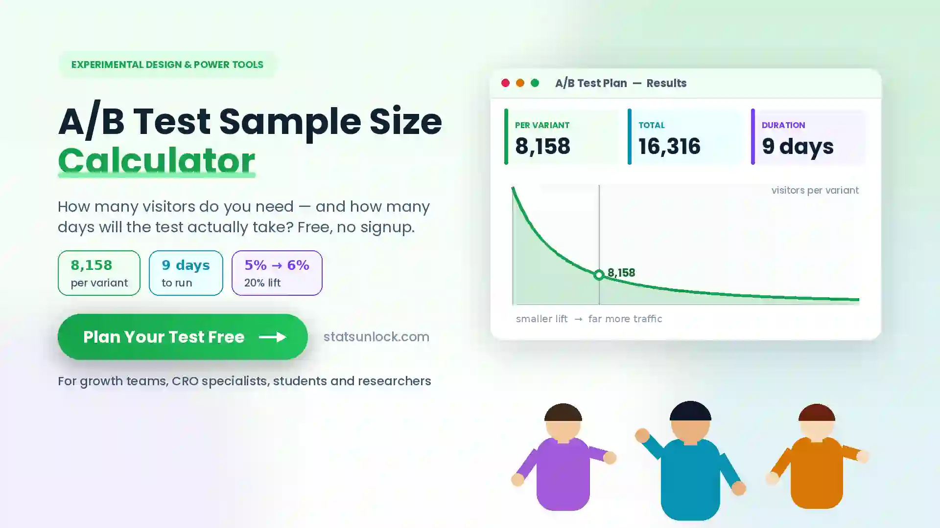
Quick answer: Sample size is driven by two numbers — your baseline conversion rate and the minimum detectable effect you care about. At a 5% baseline, detecting a 20% relative lift (5% → 6%) at 95% confidence and 80% power needs about 8,158 visitors per variant, or 16,316 total. Halve the lift you want to detect and the requirement roughly quadruples. Fix the sample size before you start, and do not stop the test early just because it looks significant.
🔑 Key Takeaways
- 1Decide the MDE first, then compute traffic. The question is not "how long should I run this?" but "what is the smallest lift worth acting on?" Everything else follows from that.
- 2Sample size scales with 1/MDE². Detecting a 10% lift needs roughly four times the traffic of a 20% lift. This single relationship kills most ambitious test plans.
- 3Low baseline rates are expensive. A 1% baseline needs far more traffic than a 10% baseline for the same relative lift, because there is less signal per visitor.
- 4Never stop at the first significant result. Peeking daily and stopping when p < .05 pushes your real false positive rate past 20%. Fix n in advance or use a sequential method.
- 5Run whole weeks. Traffic and intent vary by weekday. Stopping mid-week bakes a day-of-week bias into the result even when the sample size is met.
- 6More variants cost more than you think. Testing four variants against control means three comparisons, so alpha must be corrected and each arm still needs close to full sample size.
- 7If the required traffic is impossible, redesign the test. Target a bolder change, pick a higher-frequency metric, or test on a higher-traffic page. Do not simply run an under-powered test and hope.
1. Set Up Your Test
2. Results
Your test plan
What you could detect in a fixed runtime
Working backwards: if you can only run the test for a set number of days, this is the smallest lift you would be able to detect.
Visualisations
Sample size per variant vs the lift you want to detect
Test duration in days vs the lift you want to detect
Power gained as the test runs
How your baseline rate changes the cost
3. Interpretation of Results — In Detail
3.1 The three numbers that decide everything
An A/B test sample size is not a matter of opinion or of "how long feels right". It is determined by three inputs, and once you fix them the answer is arithmetic.
Your baseline conversion rate sets how much information each visitor carries. Binary outcomes are noisy, and they are noisiest in relative terms when the rate is low. A page converting at 1% needs far more traffic than one converting at 15% to detect the same relative improvement, because the absolute difference you are chasing is tiny.
The minimum detectable effect is the lift you want to be able to catch. This is the number teams get wrong most often. It is not the lift you hope for, and it is not the lift your last winning test produced. It is the smallest improvement that would actually change a decision — the point below which you would not bother shipping the change. Set it by asking what lift justifies the engineering and risk, not by asking what sounds impressive.
Confidence and power set your tolerance for the two ways of being wrong. Confidence of 95% means a 5% false positive rate: one in twenty tests on a genuinely useless change will look like a winner. Power of 80% means that if a real lift of your MDE size exists, you will detect it four times out of five — and miss it one time in five.
3.2 Why the traffic requirement explodes
Sample size scales with the inverse square of the effect size. Going from a 20% detectable lift to a 10% detectable lift does not double your traffic requirement — it roughly quadruples it. Going from 20% to 5% multiplies it by about sixteen.
This is the single most useful thing to internalise, because it explains why so many test plans are impossible. A team with 2,000 daily visitors and a 3% conversion rate who wants to detect a 5% relative lift is asking for about 208,000 visitors per variant — roughly seven months of uninterrupted traffic. No amount of patience fixes that. The only options are to target a bolder change, move the test to a higher-traffic page, or pick a metric that occurs more often.
The chart of sample size against MDE makes this visible. It is not a gentle slope; it is a wall. Most of the useful territory is on the right-hand side, and teams routinely plan tests deep in the impossible left-hand region without realising it.
3.3 Reading the duration figure honestly
The duration number assumes your traffic is steady and that every allocated visitor is genuinely eligible for the test. Both assumptions usually fail a little, so treat it as a floor rather than a promise. Three adjustments are worth making before you commit to a date:
- Round up to whole weeks. Conversion behaviour differs on a Tuesday and a Saturday. A test that ends mid-week over-weights whichever days it happened to include. Always run 7, 14, 21 or 28 days.
- Add a buffer for the business cycle. If your purchase cycle is two weeks, a one-week test measures only the fast converters and will misestimate the true effect.
- Account for seasonality and campaigns. A test running through Black Friday or a big email push is measuring a different population from your baseline.
If the calculated duration exceeds about four weeks, be sceptical of the whole plan. Long tests accumulate cookie deletion, cross-device contamination and product changes that quietly break the comparison.
3.4 The peeking problem
The mathematics is simple: each look is another opportunity to cross the threshold by chance, and random walks wander. A test with no real effect will drift across the significance line at some point in its run surprisingly often — and if your stopping rule is "stop when significant", you will catch it exactly at that moment.
There are only two honest options. Either fix the sample size in advance and look once at the end, which is what this calculator is designed for. Or adopt a method built for continuous monitoring — sequential testing with alpha spending, or a Bayesian approach with a pre-specified decision rule. What you cannot do is use fixed-sample statistics and a flexible stopping rule.
3.5 Decision guide
3.6 Common mistakes this calculator prevents
- Planning by calendar. "We'll run it for two weeks" is not a design. Two weeks might be five times too short or ten times too long.
- Using the hoped-for lift as the MDE. Optimism here produces a study that only detects miracles.
- Forgetting the correction for multiple variants. Testing five variants at α = .05 each gives a family-wise error rate near 19%.
- Ignoring the allocation percentage. Ramping to 10% of traffic for safety multiplies your duration by ten.
- Treating a non-significant result as "no difference". It usually means the test could never have detected the effect in question. Check the MDE.
4. How to Report Your A/B Test
4.1 The test plan (write this before launching)
That paragraph, written before launch and shared with stakeholders, prevents almost every argument that happens after a test finishes.
4.2 Reporting a winner
Report both rates with their raw counts, the relative lift with a confidence interval, and confirmation that the plan was followed. The interval matters more than the point estimate — a 21.7% lift with a range of 4% to 41% is a real finding, but the true effect could plausibly be a quarter of the headline number.
4.3 Reporting a loser or a null result
The MDE sentence is what separates a useful null report from a wasted month. "It didn't win" and "we couldn't tell" are very different conclusions.
4.4 Translating to business impact
Always carry the confidence interval into the revenue projection. A single-point revenue figure built on an uncertain lift is how testing programmes lose credibility with finance.
4.5 Reporting checklist
- Primary metric named and defined before launch, with one metric designated primary
- Baseline rate, MDE, confidence, power and required sample stated in the plan
- Actual sample reached, and confirmation the test ran to the planned end date
- Both conversion rates with raw numerators and denominators
- Relative lift with a confidence interval, not just a point estimate
- Exact p-value, and the number of comparisons if more than one variant
- Any deviation from the plan disclosed — early stops, traffic changes, bugs
- Secondary metrics flagged as exploratory, not treated as confirmatory findings
5. Formulas Used
zβ = Φ⁻¹(power)
power.prop.test.6. How to Use This Calculator
- Load a scenario that resembles your surface — checkout, signup, email, ads — to see realistic numbers immediately.
- Enter your baseline conversion rate. Use at least four weeks of recent data for the control, not an all-time average.
- Choose how to express the effect. Relative lift (a 20% improvement) is how most teams think; absolute points is how statisticians usually specify it. Toggle between them.
- Set the minimum detectable effect to the smallest lift that would actually change your decision to ship — not the lift you are hoping for.
- Enter daily visitors and allocation. Count only visitors genuinely eligible to see the change, and reduce the allocation if you are ramping cautiously.
- Set confidence and power. 95% and 80% are standard; raise power to 90% for expensive or hard-to-repeat tests.
- Add variants if testing more than one idea, and leave the Bonferroni correction on. Watch what it does to the traffic requirement.
- Read the duration and round it up to whole weeks. If it exceeds four weeks, revisit the MDE before committing.
- Check the reverse table to see what lift you could detect in one, two or four weeks — often more useful than the forward calculation.
- Download the plan and paste it into your ticket or test document before launching. Pre-registering the sample size is what makes the result trustworthy.
7. Reference Tables
7.1 Visitors needed per variant (95% confidence, 80% power, two-sided)
| Baseline rate | 5% lift | 10% lift | 20% lift | 30% lift | 50% lift |
|---|---|---|---|---|---|
| 1% | 637,010 | 163,095 | 42,693 | 19,827 | 7,750 |
| 2% | 315,206 | 80,682 | 21,109 | 9,798 | 3,826 |
| 3% | 207,938 | 53,211 | 13,914 | 6,455 | 2,518 |
| 5% | 122,124 | 31,234 | 8,158 | 3,780 | 1,471 |
| 10% | 57,763 | 14,751 | 3,841 | 1,774 | 686 |
| 15% | 36,310 | 9,257 | 2,402 | 1,106 | 424 |
| 20% | 25,583 | 6,510 | 1,683 | 772 | 294 |
| 30% | 14,856 | 3,763 | 963 | 437 | 163 |
Read across a row to see the cost of ambition. At a 5% baseline, chasing a 5% lift instead of a 20% lift costs about 15 times more traffic (122,124 versus 8,158 per variant).
7.2 What confidence and power cost
| Setting | z value | Sample size vs baseline case | When to use |
|---|---|---|---|
| 90% confidence | 1.645 | −21% | Low-risk changes, fast iteration |
| 95% confidence | 1.960 | baseline | Standard for most product tests |
| 99% confidence | 2.576 | +49% | Expensive or irreversible changes |
| 80% power | 0.842 | baseline | Standard |
| 90% power | 1.282 | +34% | Tests you cannot easily repeat |
| 95% power | 1.645 | +66% | Critical decisions only |
| One-sided test | — | −21% | Only if a negative result is genuinely irrelevant |
7.3 Family-wise error rate without correction
| Variants (incl. control) | Comparisons | FWER at α = .05 | Bonferroni α* |
|---|---|---|---|
| 2 | 1 | 5.0% | .0500 |
| 3 | 2 | 9.8% | .0250 |
| 4 | 3 | 14.3% | .0167 |
| 5 | 4 | 18.5% | .0125 |
| 6 | 5 | 22.6% | .0100 |
8. Example Results
Six planning situations you can reproduce with the controls above.
Example 1 — The standard e-commerce checkout test
Baseline 5%, detect a 20% relative lift, 95% confidence, 80% power, 2,000 visitors/day.
Sample: 8,158 per variant (16,316 total)
Duration: 9 days → round up to 14 days
Comfortably runnable. Note the rounding: the maths says 9 days, but running two full weeks removes day-of-week bias and costs almost nothing.
Example 2 — The test nobody can afford to run
Baseline 3%, detect a 5% relative lift, same settings, 2,000 visitors/day.
Sample: 207,938 per variant (415,876 total)
Duration: 208 days ≈ 7 months
The instinct is to run it anyway and "see what happens". Do not. Either target a bolder change or accept that a 5% lift is undetectable at this traffic level and stop planning around it.
Example 3 — The cost of halving your MDE
Baseline 5%, comparing a 20% versus a 10% detectable lift.
10% lift → 31,234 per variant
Ratio: 3.8× more traffic for half the sensitivity
The inverse-square law in action. Before asking for four times the traffic, ask whether a 10% lift would really change your decision when a 20% lift would not.
Example 4 — Adding variants is expensive
Baseline 5%, 20% lift, comparing a simple A/B against a four-variant test with Bonferroni.
4 variants (α = .0167): 10,882 each → 43,528 total
Total traffic needed: 2.7× more
Two effects compound: the corrected alpha raises the per-variant requirement, and you need that sample in more arms. Test fewer, bolder ideas.
Example 5 — Ramping traffic multiplies duration
Baseline 5%, 20% lift, 2,000 visitors/day, but only 25% allocated to the experiment.
Effective daily traffic: 500 instead of 2,000
Duration: 33 days instead of 9
A cautious ramp is sensible for risky changes, but it is a direct multiplier on runtime. Ramp for the first days, then move to full allocation.
Example 6 — Working backwards from a deadline
You have 14 days and 2,000 visitors/day at a 5% baseline. What can you actually detect?
Detectable lift: 15.1% relative (5% → 5.76%)
Anything smaller will likely be missed
This reverse calculation is usually more useful than the forward one, because deadlines are typically fixed and MDEs are not. If a 15% lift is not worth shipping, the test is not worth running.
9. When to Use This Calculator
Use it before launching any A/B test on a binary outcome — conversion rate, click-through rate, signup rate, checkout completion, email open or click, app install, trial start, or any other yes/no event. Use it when a stakeholder asks "how long will this take?", when you need to justify why a test cannot detect a 2% lift, when deciding between testing two ideas or five, and when working backwards from a fixed deadline to see what is realistically detectable.
It suits growth and product teams, conversion rate optimisation specialists, marketers running landing page tests, data analysts reviewing test plans, and students learning experimental design with a practical example.
Use something else when: your metric is continuous rather than binary — revenue per visitor, time on page, average order value — in which case use the Statistical Power Analysis Calculator with Cohen's d; when you need sequential or Bayesian testing that allows continuous monitoring; when your unit of randomisation is a cluster such as a store or a city; or when you are running a multi-armed bandit, which optimises allocation rather than testing a fixed hypothesis.
10. Assumptions and Limitations
- Binary outcome. Each visitor either converts or does not. Revenue, order value and time-based metrics need a different formula.
- Normal approximation. The standard two-proportion formula assumes large enough samples that the normal approximation holds. It becomes unreliable when the expected number of conversions per variant falls below about 30 — with very low rates or tiny samples, use an exact test.
- Independent visitors. Each visitor is counted once and assigned to one variant. Cross-device usage, shared computers and cookie deletion all violate this and dilute the measured effect.
- Stable traffic and behaviour. Duration assumes constant daily visitors. Seasonality, campaigns and product releases during the test change the population being measured.
- Even traffic split. Sample size is per variant under equal allocation, which is the most efficient design. Unequal splits need more total traffic for the same power.
- One primary metric. Testing many metrics is another multiplicity problem. Nominate one primary metric in advance and treat the rest as exploratory.
- Fixed-sample statistics. These formulas assume you look once, at the end. They are invalid under repeated peeking with an early-stopping rule.
- Bonferroni is conservative. For many variants it over-corrects. Dunnett's procedure or false discovery rate control are more efficient when comparing several variants against one control.
- The MDE is a planning input, not a prediction. Powering for a 20% lift does not mean you will observe one.
11. Conclusion
Most failed A/B testing programmes do not fail because the ideas were bad. They fail because the tests were never capable of answering the question. A team runs a two-week test on a low-traffic page, sees no significant difference, concludes the idea did not work, and moves on — when in fact the test could only ever have detected a lift three times larger than anything realistic. Calculating the sample size in advance converts that invisible failure into a visible decision you can make before spending the month.
The arithmetic is unforgiving in one specific way that is worth memorising: sample size scales with the inverse square of the effect you want to detect. Halve the MDE and you need roughly four times the traffic. This is why small optimisations are so expensive to verify, why low-converting pages are hard to test on, and why the most productive testing programmes tend to test bold changes rather than button colours. If your traffic cannot support the test you want, the honest responses are to test something bolder, move to a higher-traffic surface, choose a more frequent metric, or accept that this particular question is not answerable with the traffic you have.
The second lesson is about discipline after launch. Fixed-sample statistics assume a single look at a pre-specified endpoint. Checking daily and stopping at the first significant result is not a minor shortcut — it can quadruple your false positive rate, and it does so invisibly, producing confident-looking winners that quietly fail to replicate. Either commit to the sample size and the end date, or switch to a sequential or Bayesian method built for continuous monitoring. Choosing one of those two options, and writing it down before launch, is the single highest-return habit in experimentation.
Finally, treat the reverse calculation as your default. Deadlines are usually fixed and traffic is usually what it is, so the practical question is rarely "how long do I need?" but "given two weeks, what could I actually detect, and is that worth knowing?" If the answer is that you could only detect a 25% lift and no realistic change will produce one, you have saved yourself a month and learned something useful before writing a line of code.
12. Frequently Asked Questions
How many visitors do I need for an A/B test?
It depends on your baseline rate and the lift you want to detect. At a 5% baseline detecting a 20% relative lift at 95% confidence and 80% power, you need about 8,158 per variant. At a 1% baseline it is about 42,700 per variant for the same relative lift.
How long should an A/B test run?
Long enough to reach the required sample, rounded up to whole weeks, and never less than one full business cycle. Two weeks is a common practical minimum even when the sample arrives sooner.
Can I stop the test as soon as it hits significance?
No. Peeking and stopping early inflates the false positive rate from 5% to roughly 20–30%. Either fix the sample in advance or use a sequential method designed for monitoring.
What is a minimum detectable effect?
The smallest lift your test can reliably detect at your chosen confidence and power. It is a design input, not a prediction of what you will observe.
Should I use relative or absolute lift?
Relative lift (20% better) is how most teams reason and communicate. Absolute points (5% → 6%) is unambiguous and preferred in formal write-ups. This calculator does both — just be explicit about which you mean.
What MDE should I choose?
The smallest improvement that would change your decision to ship. If a 10% lift would not justify the engineering effort, do not power for 10%.
Why does a low conversion rate need so much traffic?
Binary outcomes carry little information each, and at low rates the absolute difference you are chasing is tiny. Going from 1% to 1.2% is a 20% relative lift but only 0.2 percentage points of signal.
Is 95% confidence and 80% power always right?
They are sensible defaults, not rules. Lower confidence to 90% for cheap reversible changes; raise power to 90% for tests you cannot repeat.
Should I use a one-sided or two-sided test?
Two-sided in almost all cases. One-sided saves about 21% of your traffic but commits you to ignoring a result in the opposite direction — and knowing that a change actively hurt conversion is usually valuable.
How do I handle more than two variants?
Correct alpha for the number of comparisons against control and expect a substantially larger total sample. Four variants needs roughly 2.7 times the total traffic of a simple A/B.
What if my traffic is uneven between variants?
Power is governed by the harmonic mean of the group sizes, so an uneven split wastes data. Use a 50/50 split whenever you can.
Does allocating less traffic change the sample size?
No — the sample size stays the same, but the duration stretches proportionally. Allocating 25% of traffic makes the test take four times as long.
What is the novelty effect?
Regular users react to a change simply because it is new, inflating early results. It is one reason short tests mislead and why running at least one full business cycle matters.
What if the test finishes and the result is not significant?
Report it as inconclusive and state the MDE. It usually means the true effect is smaller than what you powered for, not that there is no effect.
Can I extend a test that just missed significance?
Not without invalidating the statistics. Extending because you did not like the result is a form of peeking. Plan a fresh, properly powered test instead.
Should I test multiple metrics?
Nominate one primary metric in advance. Monitor others as guardrails or exploratory signals, but do not declare a winner based on whichever metric happened to reach significance.
What is the difference between an A/B test and a multi-armed bandit?
An A/B test answers a question with a fixed sample and clean statistics. A bandit maximises reward during the test by shifting traffic to the leader, which is better for short campaigns but gives weaker inference.
How does this compare with Evan Miller's or Optimizely's calculator?
The core formula is the same standard two-proportion calculation and matches R's power.prop.test. This tool adds test duration, multi-variant correction, and the reverse MDE calculation in one place.
Do I need to worry about the normal approximation?
Only with very low rates or very small samples. As a rule of thumb, if the expected conversions per variant exceed about 30 you are fine; below that, use an exact test.
What sample size do I need to detect a 1% relative lift?
Usually an impractical one. At a 5% baseline it is around 3 million visitors per variant. Very small lifts are effectively unmeasurable outside enormous-traffic sites.
Can I run the test on a percentage of traffic to be safe?
Yes, and it is good practice for risky changes — just remember it multiplies the duration by the inverse of the allocation.
Does statistical significance mean the result is worth shipping?
No. Significance says the effect is unlikely to be zero; it says nothing about whether the effect is big enough to matter. Check the confidence interval against your minimum worthwhile effect.
13. Cite This Tool
Free to use and free to reference. If this calculator helped plan a test, a citation or link is appreciated.
StatsUnlock. (2026). A/B Test Sample Size Calculator [Interactive statistical tool]. https://statsunlock.com/ab-test-sample-size-calculator/
@misc{statsunlock_abtest_2026,
  title  = {A/B Test Sample Size Calculator},
  author = {{StatsUnlock}},
  year   = {2026},
  note   = {Interactive statistical tool},
  url    = {https://statsunlock.com/ab-test-sample-size-calculator/}
}
Sample size was determined in advance using the StatsUnlock A/B Test Sample Size Calculator (statsunlock.com), based on the observed baseline conversion rate and the minimum detectable effect agreed with stakeholders. No interim significance testing was performed.
14. Related Tools
Part of the StatsUnlock experimental design toolkit — all free, no signup, and they work together.
Effect size, achieved power, required sample size per group and the minimum detectable effect for t-tests and one-way ANOVA.
Open the tool →See alpha, beta and power as areas under two curves, and find out how often a significant result is actually false.
Open the tool →