


Type I & Type II Error Explorer
Move alpha, effect size and sample size and watch the two hypothesis curves, the false positive and false negative regions, and the false discovery rate update instantly. The picture every statistics course draws — made interactive.
Quick answer: A Type I error is a false positive — rejecting a true null hypothesis. Its rate is α, which you choose (usually 0.05). A Type II error is a false negative — missing a real effect. Its rate is β, and power = 1 − β. At a fixed sample size the two trade off: lowering α raises β. Only more data, a larger effect, or less measurement noise reduces both at once. And when most tested hypotheses are false, even a correct α = 0.05 can still leave most significant findings wrong — that is the false discovery rate.
🔑 Key Takeaways
- 1Type I error = false positive = α. You set it before the study. It is the long-run rate of crying wolf when nothing is happening.
- 2Type II error = false negative = β. You do not set it directly — it falls out of your alpha, effect size and sample size. Power is its complement.
- 3α and β trade off at a fixed n. Moving the critical value to catch fewer false positives inevitably lets more real effects slip through.
- 4Only sample size, effect size or lower noise beat the trade-off. They pull the two curves apart, shrinking both error rates at once.
- 5α is not the chance your significant result is wrong. That is the false discovery rate, and it depends on how often the hypotheses you test are actually true.
- 6In low-prior fields, most significant findings are false. With a 10% prior, α = .05 and 80% power, over a third of your "discoveries" are false positives.
- 7Choose α and β by consequence, not convention. Ask what a false alarm costs versus a missed effect, then set the rates to match.
1. Set Your Study Parameters
2. Results
The two hypothesis distributions
Decision matrix — what happens in 1000 studies
Full results table
Visualisations
Outcome breakdown of every study run
The α / β trade-off at your sample size
False discovery rate vs how often H₁ is true
3. Interpretation of Results — In Detail
3.1 What the two curves actually represent
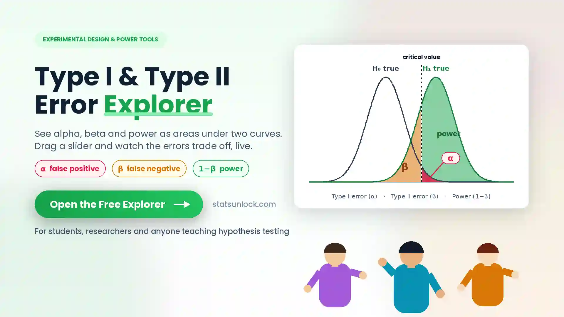
The chart shows two sampling distributions of the same test statistic. The left curve is what you would see if the null hypothesis were true — no effect, only sampling noise. The right curve is what you would see if the alternative were true at the effect size you specified. The vertical line is the critical value: any result to the right of it gets called significant.
Everything follows from where that line sits. The slice of the null curve beyond the line is α, the Type I error rate — results that look significant even though nothing is going on. The slice of the alternative curve on the wrong side of the line is β, the Type II error rate — real effects that fail to reach significance. What remains of the alternative curve is power.
Drag the alpha slider and watch the line move. Push it right to shrink the red area and the amber area grows; push it left and the reverse happens. That is the trade-off in its purest form: at a fixed sample size, you cannot reduce both errors at once. Now drag the sample size slider instead. The alternative curve slides away from the null, and red and amber shrink together. Sample size is the only lever that buys you both.
3.2 The number most people get wrong
Alpha is not the probability that a significant finding is a false alarm. Alpha is conditional on the null being true: given no effect, 5% of studies will cross the threshold. The question researchers actually care about runs the other way — given that I got a significant result, how likely is it to be real? That is the positive predictive value, and its complement is the false discovery rate.
Answering it requires one extra ingredient the p-value cannot supply: how often the hypotheses you test are true in the first place. Set the prior slider to 0.50 with α = .05 and 80% power and the false discovery rate is about 6% — comfortable. Now drop the prior to 0.10, the realistic figure for exploratory screening, and it jumps past 35%. Drop power to 0.35, typical of a small study, and more than half of your significant findings are false, even though your alpha never changed.
This is why the replication crisis is not mainly a story about fraud. Low prior probability plus low power plus a 0.05 threshold produces a large false discovery rate automatically, and every one of those false positives looks exactly like a real finding on paper.
3.3 Reading the four visuals
The distribution chart is the one to put in a lecture slide or a thesis. It makes the definitions concrete: α and β are areas, not abstractions, and they live on different curves. Note that they are areas under different distributions — a common student error is to think they must sum to one.
The decision matrix converts the rates into counts. Rates are easy to nod along to; "of 1000 studies, 45 were false alarms and 20 were missed effects" is much harder to misread. This framing also makes the asymmetry visible — in most realistic settings there are far more true nulls than true effects, so even a small α produces a lot of false positives in absolute terms.
The trade-off curve plots β and power against every possible alpha at your current sample size. The crossing point shows where the two error rates are equal, which some fields use as a principled alternative to the 0.05 convention. The curve is steep at small alpha: tightening from .05 to .01 costs a lot of power, tightening from .01 to .001 costs less again.
The false discovery curve plots FDR against the prior. It falls sharply as the prior rises, which is the quantitative case for testing well-motivated hypotheses rather than fishing. Two studies with identical alpha and power can have wildly different credibility depending only on how plausible the hypothesis was before the data arrived.
3.4 Decision guide
3.5 Choosing α and β by consequence
The 0.05 convention is a historical accident that Fisher proposed as a rough working rule, and 0.80 power comes from Cohen's judgement that a Type II error is roughly four times less costly than a Type I. Neither is a law. The honest approach is to ask what each mistake actually costs in your setting.
- False positive expensive (drug approval, criminal conviction, particle discovery): tighten α. Physics uses 5-sigma, about 0.0000003.
- False negative expensive (disease screening, safety testing, conservation triage): protect power first, and accept a looser α. Missing a declining population is worse than a needless extra survey.
- Both expensive: the only real answer is more data or better measurement. Blocking, covariates and reliable instruments shrink noise and move both curves apart.
- Many tests at once: correct α for multiplicity, but budget the sample size increase that keeps power intact, or you have simply traded false positives for false negatives.
4. How to Write Your Results in Research
4.1 Stating the error rates in the Methods
Name both rates explicitly. Reviewers notice when β is never mentioned, because it signals the Type II error was never considered.
4.2 Justifying a non-standard alpha
This sentence does more for a methods section than any amount of defending 0.05. It shows the threshold was a decision, not a default.
4.3 Reporting a multiplicity correction
4.4 Interpreting a non-significant result correctly
Quoting β for the effect you cared about is what converts "we found nothing" into a statement a reader can evaluate.
4.5 Discussing the false discovery rate
Very few papers include a sentence like this, and it is exactly the kind of calibrated honesty that reviewers and meta-scientists reward.
4.6 Checklist
- α stated with the test direction (one- or two-tailed) and justified if non-standard
- β or power stated, with the effect size it refers to
- Effect size reported with a 95% confidence interval, not just a p-value
- Multiplicity correction named, with its effect on power addressed
- Non-significant results described as inconclusive unless an equivalence test was run
- Exploratory versus confirmatory analyses clearly separated
- Statistical symbols italicised: α, β, p, d, n
5. Formulas Used
zcrit = Φ⁻¹( 1 − α ) one-tailed
λ = d · √n one sample
β = 1 − Power
FP = N·(1−π)·α TN = N·(1−π)·(1−α)
6. How to Use This Explorer
- Start with a scenario. Pick one from the dropdown to load a realistic combination of parameters and see immediately what it implies.
- Set your alpha. The slider moves the critical line on the chart. Watch the red Type I area change as you drag.
- Set the effect size you care about. This is the smallest difference worth detecting, not the one you hope to find. It slides the alternative curve.
- Set your sample size. Larger n narrows both distributions, pulling them apart and shrinking both error regions at once.
- Set the prior. How often are hypotheses like yours actually true? Confirmatory work might be 0.5 or higher; broad exploratory screening is closer to 0.05.
- Read the KPI cards for α, β, power, false discovery rate and positive predictive value.
- Read the decision matrix to see those rates as counts of real studies — the framing that makes the numbers click.
- Check the trade-off chart to see what a different alpha would cost you in power at this sample size.
- Check the FDR curve to see how much the credibility of a significant finding depends on the plausibility of the hypothesis.
- Download the figure as a PNG for your slides or thesis, and the numbers as a .txt for your notes.
7. Reference Tables
7.1 Critical values and Type I error rates
| Alpha | z (two-tailed) | z (one-tailed) | False positives per 1000 true nulls | Typical use |
|---|---|---|---|---|
| 0.10 | 1.645 | 1.282 | 100 | Screening, ecology where misses are costly |
| 0.05 | 1.960 | 1.645 | 50 | Default convention across most fields |
| 0.01 | 2.576 | 2.326 | 10 | Confirmatory studies, stricter journals |
| 0.005 | 2.807 | 2.576 | 5 | Proposed new default for claims of discovery |
| 0.001 | 3.291 | 3.090 | 1 | Genomics, large multiple-testing settings |
| 0.0000003 | 5.000 | 4.750 | 0.0003 | Particle physics 5-sigma standard |
7.2 Type II error rate (β) by power
| Power (1 − β) | β | Real effects missed per 100 | Verdict |
|---|---|---|---|
| 0.50 | 0.50 | 50 | Coin flip — inadequate |
| 0.60 | 0.40 | 40 | Under-powered |
| 0.70 | 0.30 | 30 | Marginal |
| 0.80 | 0.20 | 20 | Conventional target |
| 0.90 | 0.10 | 10 | Strong, common for confirmatory work |
| 0.95 | 0.05 | 5 | Very strong, expensive |
7.3 False discovery rate at α = 0.05
| Prior P(H₁) | Power 0.30 | Power 0.50 | Power 0.80 | Power 0.95 |
|---|---|---|---|---|
| 0.01 | 94.3% | 90.8% | 86.1% | 83.9% |
| 0.05 | 76.0% | 65.5% | 54.3% | 50.0% |
| 0.10 | 60.0% | 47.4% | 36.0% | 32.1% |
| 0.25 | 33.3% | 23.1% | 15.8% | 13.6% |
| 0.50 | 14.3% | 9.1% | 5.9% | 5.0% |
| 0.80 | 4.0% | 2.4% | 1.5% | 1.3% |
Read this table once and the replication crisis stops being mysterious. A field testing long-shot hypotheses with small samples produces mostly false positives while following every rule correctly.
8. Example Results
Six scenarios you can reproduce with the sliders above.
Example 1 — The textbook design
α = .05 two-tailed, d = 0.50, n = 64 per group, prior = 0.50.
Of 1000 studies: 404 true positives, 25 false positives, 96 missed effects
False discovery rate = 5.8% · PPV = 94.2%
The balanced case everything else is measured against. A significant result here is trustworthy — but note that it took a 50% prior to get there.
Example 2 — The under-powered study
α = .05, d = 0.30, n = 20 per group, prior = 0.50.
Of 1000 studies: 79 true positives, 25 false positives, 421 missed effects
False discovery rate = 24.1%
More than five real effects are missed for every one detected. Worse, almost a quarter of the "successes" are false alarms — and because only unusually large sample effects clear the threshold at this n, the published effect sizes will also be badly inflated.
Example 3 — Tightening alpha without adding data
Same as Example 1 but α = .001.
False discovery rate = 0.3%
False positives nearly vanish, but power collapses from 0.81 to 0.32. This is the trade-off at its starkest: you have not made the study better, you have moved the error from one column to the other. Only a larger n buys both.
Example 4 — Exploratory screening
α = .05, d = 0.50, n = 64, but prior = 0.05.
Of 1000 studies: 40 true positives, 48 false positives
Nothing about the test changed — same alpha, same power — yet the majority of significant results are now false. The credibility of a finding depends on the plausibility of the hypothesis, which no p-value can tell you.
Example 5 — Paying for a multiplicity correction
Six comparisons, Bonferroni α = .0083, d = 0.50, n = 64.
Raising n to 97 per group restores power to 0.800
Correcting for multiplicity is right, but doing it without increasing n silently converts a well-powered study into an under-powered one. Budget the extra participants at the design stage.
Example 6 — When a false negative is the expensive error
Conservation monitoring: α = .10 one-tailed, d = 0.40, n = 30.
At α = .05 the same design gives power = 0.462
Relaxing alpha lifts power by 14 points. If failing to detect a declining population costs more than an unnecessary follow-up survey, that is the correct trade — and saying so explicitly is far stronger than defending 0.05 by habit.
9. When to Use This Tool
Use this explorer when you are teaching or learning hypothesis testing and need the α/β picture to become concrete; when you are choosing a significance threshold and want to see what it costs in power; when a reviewer asks you to justify alpha; when you are deciding whether a multiplicity correction needs a larger sample; when you want to explain to a collaborator why a significant result from an exploratory screen is weak evidence; or when you are building slides and need a clean, correct figure of the two hypothesis distributions.
It suits students meeting Type I and Type II errors for the first time, lecturers who want a live demonstration rather than a static slide, researchers writing a methods section, and anyone trying to explain the replication crisis with numbers instead of adjectives.
Use something else when: you need an exact sample size for a specific test — use the Statistical Power Analysis Calculator, which uses the exact noncentral t and F distributions; or when your design has repeated measures, nesting or non-normal outcomes, which need simulation-based methods.
10. Assumptions and Limitations
- Normal (z) approximation. The curves and areas use the standard normal distribution, which is what every textbook figure shows and keeps the shaded areas exactly equal to the reported α, β and power. For small samples the exact t-based power is slightly lower; the results panel reports both so you can see the gap.
- A single specified effect size. Beta and power are defined only relative to one assumed effect. There is no such thing as "the" Type II error rate of a study without naming the effect it refers to.
- Independence and equal variances. The standard two-sample framing is assumed. Clustering, repeated measures or strongly unequal variances change the effective sample size.
- The prior is a judgement, not a measurement. The false discovery rate depends on how often hypotheses like yours are true, which you must estimate from field knowledge. Treat it as a sensitivity analysis: try 0.05, 0.25 and 0.50 and see whether your conclusion survives.
- One test at a time. The decision matrix assumes each study is a single independent test. Multiple testing within a study inflates the effective alpha unless corrected.
- No publication bias. Real literatures filter which results appear, which raises the observed false discovery rate above the figure computed here.
- Equal group sizes. With unequal groups, power is governed by the harmonic mean of the sample sizes.
- Type S and Type M errors are not modelled. Under-powered significant results are also frequently exaggerated in magnitude, and occasionally wrong in sign — a separate problem from the Type I/II framework.
11. Conclusion
Type I and Type II errors are usually taught as a pair of definitions to memorise, which is why so many people can recite them and still misuse them. Seen as areas under two curves, they become obvious: the null distribution and the alternative distribution overlap, a threshold has to be drawn somewhere in that overlap, and wherever you draw it you are choosing how to split your mistakes between false alarms and missed effects.
The single most useful thing this explorer shows is that the trade-off is not symmetric in your control. Alpha is a dial you set directly. Beta is not — it is the downstream consequence of that dial together with your effect size and your sample size. Researchers who obsess over the significance threshold while ignoring sample size have optimised the one error they can see and left the other to chance. Moving the threshold shuffles risk between the two columns; only more data, a bigger effect, or less measurement noise reduces both.
The second lesson is the one the classic 2×2 table hides. Alpha answers "how often will I be fooled when nothing is there?" — a question about a world you are not in, because you do not know whether the null is true. The question you actually face is "given that I found something, how likely is it to be real?", and answering it requires knowing how often hypotheses like yours turn out to be true. That is why a significant result from a well-motivated confirmatory test and a significant result from a broad exploratory screen are not equally believable, even with identical p-values. The false discovery rate makes the difference explicit, and it explains most of the replication crisis without needing to invoke misconduct at all.
Practically, three habits follow. Choose alpha by consequence rather than convention, and say in your methods why you chose it. Design for power against the smallest effect that would matter, and report beta when your result is null. And before believing your own significant finding, ask honestly how plausible the hypothesis was beforehand — then look at what that implies for the false discovery rate.
12. Test Yourself
Twenty-three questions covering the mistakes people actually make — definitions, the trade-off, multiplicity, and the false discovery rate. Each answer explains the reasoning, not just the letter.
13. Frequently Asked Questions
What is a Type I error in simple terms?
A false positive: you conclude there is an effect when there is not. The classic analogy is a smoke alarm going off when there is no fire. Its long-run rate is alpha.
What is a Type II error in simple terms?
A false negative: a real effect exists and your study misses it. The smoke alarm that stays silent during a fire. Its rate is beta.
Which error is worse?
Whichever costs more in your context. Approving an ineffective drug is a costly Type I error; missing an early cancer is a costly Type II error. Set alpha and power to reflect those costs rather than defaulting to .05 and .80.
How do I remember which is which?
Type I has one letter in "false positive" order — you assert something that is not there. A common mnemonic: Type I = "seeing something that isn't there", Type II = "missing something that is".
Do alpha and beta add up to 1?
No, and this is the most common misunderstanding. They are areas under two different distributions. Alpha lives on the null curve, beta on the alternative curve. Only beta and power sum to 1.
Why does lowering alpha increase beta?
Lowering alpha pushes the critical value further into the tail. That shrinks the null curve's tail area, but it also puts more of the alternative curve on the non-significant side, so more real effects are missed.
How do I reduce both errors at once?
Increase the sample size, study a larger effect, or reduce measurement noise. All three separate the two distributions, shrinking both error regions simultaneously. Moving the threshold cannot do this.
Is alpha the probability that my significant result is wrong?
No. Alpha is conditional on the null being true. The probability your significant result is wrong is the false discovery rate, which also depends on the prior probability that your hypothesis is true.
What is the false discovery rate?
The proportion of your significant findings that are actually false positives. With a 10% prior, alpha of .05 and 80% power it is about 36% — far higher than most researchers assume.
What is positive predictive value?
The complement of the false discovery rate: the probability that a significant result reflects a real effect. This is the number people usually think a p-value gives them.
Why is 0.05 the standard alpha?
Fisher suggested it as a convenient rough threshold, and it stuck. It is a convention, not a mathematical result. Several fields have proposed 0.005 for claims of new discoveries; particle physics uses about 0.0000003.
Why is 0.80 the standard power?
Cohen proposed it, reasoning that a Type II error is roughly four times less costly than a Type I error at alpha .05. Like 0.05, it is a default rather than a rule, and confirmatory work often targets 0.90 or 0.95.
What is the Type II error rate of my study?
The question is incomplete without an effect size. Beta is always relative to a specific alternative — a study can have beta of .05 for a large effect and .80 for a small one at the same time.
How does multiple testing affect Type I errors?
Each test carries its own alpha, so the chance of at least one false positive grows quickly: with 20 independent tests at .05 it is about 64%. Corrections like Bonferroni or FDR control fix this, but reduce power unless you also increase n.
What is the difference between family-wise error rate and false discovery rate?
The family-wise error rate is the probability of making at least one Type I error across a set of tests, controlled by Bonferroni-type methods. The false discovery rate is the expected proportion of significant results that are false, controlled by Benjamini-Hochberg, and is less conservative.
Can I have a low Type I and low Type II error rate?
Yes, but only by increasing the sample size or the effect size. At a fixed n the two are locked in a trade-off.
What is a Type III error?
An informal term for correctly rejecting the null but getting the direction of the effect wrong, or for answering the wrong question entirely. Gelman and Carlin call the sign version a Type S error.
What are Type S and Type M errors?
Type S is getting the sign of the effect wrong; Type M is exaggerating its magnitude. Both are common in under-powered studies, because only unusually extreme sample results reach significance.
How does this relate to sensitivity and specificity?
Directly. Power is sensitivity (true positive rate) and 1 − alpha is specificity (true negative rate). The false discovery rate here is the same calculation used for diagnostic tests, with the prior playing the role of disease prevalence.
Does a non-significant result mean there is no effect?
No. It means the data were insufficient to detect one. Report beta or the minimum detectable effect, and use an equivalence test if you want to argue for the absence of a meaningful effect.
Why does this tool use the normal distribution instead of the t?
So the shaded areas exactly match the reported alpha, beta and power, which is what makes the figure a correct teaching illustration. The exact t-based power is also reported for comparison, and is typically within 1 to 2 percentage points.
Can I use the figure in my thesis or lecture slides?
Yes. Use the "Download main figure" button for a PNG. A citation back to statsunlock.com is appreciated but not required.
14. Cite This Tool
Free to use and free to reuse. If this explorer or its figure helped your teaching, thesis or paper, a citation is appreciated — and the downloadable figure may be reproduced with attribution.
StatsUnlock. (2026). Type I & Type II Error Explorer [Interactive statistical tool]. https://statsunlock.com/type-1-type-2-error-explorer/
"Type I & Type II Error Explorer." StatsUnlock, 2026, statsunlock.com/type-1-type-2-error-explorer/.
@misc{statsunlock_type12_2026,
  title  = {Type I and Type II Error Explorer},
  author = {{StatsUnlock}},
  year   = {2026},
  note   = {Interactive statistical tool},
  url    = {https://statsunlock.com/type-1-type-2-error-explorer/}
}
Figure 1. Type I and Type II errors. The null (H0) and alternative (H1) sampling distributions with the critical value marked. Red = Type I error rate (alpha), amber = Type II error rate (beta), green = statistical power (1 - beta). Figure generated with the StatsUnlock Type I & Type II Error Explorer (statsunlock.com).
Methods-section wording: "Error rates and the false discovery rate were computed using the StatsUnlock Type I & Type II Error Explorer (statsunlock.com)."