Leptokurtic vs Platykurtic: Free Kurtosis Calculator & Guide

Leptokurtic vs Platykurtic: Kurtosis Calculator with Plots & Interpretation

Paste your data or upload a CSV file and instantly find out whether your distribution is leptokurtic (heavy tails), platykurtic (light tails), or mesokurtic (normal-like). Get the excess kurtosis, standard error, four colorful plots, and ready-to-copy sentences for your research paper.

Descriptive StatisticsKurtosisTail WeightFree Online Tool

Quick answer: Kurtosis measures how heavy the tails of a distribution are — how prone your data are to extreme outliers. A leptokurtic distribution has excess kurtosis above 0 (heavier tails than normal, more outliers). A platykurtic distribution has excess kurtosis below 0 (lighter tails, fewer outliers). A mesokurtic distribution has excess kurtosis near 0, like the normal distribution.

🔑 Key Takeaways

1Kurtosis is about the tails, not the peak. High kurtosis means heavy tails and frequent extreme values; the popular "peakedness" definition is a misconception (Westfall, 2014).
2The normal distribution scores kurtosis = 3, or excess kurtosis = 0. Almost all software (SPSS, Excel, R) reports excess kurtosis, so 0 is your reference point, not 3.
3Leptokurtic = excess kurtosis > 0. Heavy tails, sharp center, and outliers far more common than a normal distribution predicts — think stock returns and reaction times.
4Platykurtic = excess kurtosis < 0. Light tails and almost no outliers — the uniform distribution (excess kurtosis −1.2) is the textbook case. The mathematical floor is −2.
5Test significance with z = G₂ ÷ SEK. If |z| > 1.96 the kurtosis differs significantly from normal at α = 0.05 — but at large n, judge by the value and plots instead.
6Excess kurtosis within ±1 is fine for most parametric tests; within ±2 is usually tolerable; beyond that, outlier-robust methods, transformations, or heavy-tailed models are safer.
7Always check kurtosis together with skewness. A symmetric distribution can still be violently non-normal through its tails — normality requires both statistics near zero plus a Q-Q plot check.

📥 Enter Your Data

Comma-separated input is the default. You can also separate values with spaces, semicolons, or new lines. The group name is editable — click it and type your own label.

Upload CSV file (.csv, .txt)

Headers are detected automatically. Click the columns that should each become a cluster — every selected column is loaded as its own separate group.

🛠 How to Use This Kurtosis Calculator

Enter your data. Paste comma-separated values (e.g., 52, 48, 55, 61, 47), load one of the five sample datasets, or upload a CSV file and click the columns you want loaded as separate clusters.
Name your groups. Click any group name to edit it, and use + Add Group to compare several variables side by side.
Click "Calculate Kurtosis." The tool computes the excess kurtosis g₂, the adjusted G₂ (matches SPSS, Excel, and R), the standard error of kurtosis, and the z-test.
Read the tail weight. Excess kurtosis > 0 means leptokurtic (heavy tails); < 0 means platykurtic (light tails); within ±1 is approximately mesokurtic.
Verify with the plots and report. Check the histogram, box plot, normal-overlay plot, and Q-Q plot, then copy an APA-style template from the reporting section into your paper.

↔ Leptokurtic vs Platykurtic vs Mesokurtic: The Core Difference

The fastest way to understand kurtosis is this: kurtosis measures the tails, not the peak. A leptokurtic distribution produces extreme values far more often than a normal distribution — its tails are heavy, or "fat." A platykurtic distribution almost never produces extreme values — its tails are light and thin. The normal distribution sits exactly in between and is called mesokurtic. Whether you compare a leptokurtic vs platykurtic distribution, heavy tailed vs light tailed distributions, or positive kurtosis vs negative kurtosis, the answer always lives in the tails.

Feature	Leptokurtic (Positive)	Mesokurtic (Normal)	Platykurtic (Negative)
Excess kurtosis	Greater than 0	About 0	Less than 0 (floor: −2)
Raw kurtosis	Greater than 3	About 3	Less than 3
Tails	Heavy / fat — outliers common	Normal weight	Light / thin — outliers rare
Typical shape	Sharp center, long tails	Classic bell curve	Broad, flat-ish top
Real examples	Stock returns, insurance claims, reaction times	Heights, measurement errors	Uniform data, bounded ratings, lottery numbers
Textbook model	Student's t (low df), Laplace	Normal (Gaussian)	Uniform (excess = −1.2)

The word "kurtosis" comes from the Greek kyrtos, meaning curved or arched. "Lepto-" means slender, "platy-" means broad, and "meso-" means middle — but remember the names describe the historical (and misleading) peak-shape intuition; the modern, correct reading is always tail weight.

ƒ Formulas Used

①

Sample Mean

x̄ = Σxᵢ ÷ n

xᵢEach individual value in your dataset

nNumber of observations in the group

②

Central Moments (Second and Fourth)

m₂ = Σ(xᵢ − x̄)² / n m₄ = Σ(xᵢ − x̄)⁴ / n

m₂Second central moment — the (population) variance

m₄Fourth central moment — heavily dominated by extreme deviations, which is why kurtosis reads the tails

③

Excess Kurtosis (g₂)

g₂ = ( m₄ ÷ m₂² ) − 3

g₂Moment-based excess kurtosis — positive means leptokurtic, negative means platykurtic

−3Subtracting 3 centres the normal distribution at zero, giving "excess" kurtosis

④

Adjusted Kurtosis (G₂) — SPSS / Excel / R default

G₂ = [ (n+1) g₂ + 6 ] × (n−1) ÷ [ (n−2)(n−3) ]

G₂Small-sample bias-corrected excess kurtosis reported by SPSS, Excel (KURT), and R (type 2)

Rule|G₂| < 1 approx. normal tails · 1–2 moderate · > 2 strong departure

⑤

Standard Error of Skewness (building block)

SES = √[ 6n(n − 1) ÷ ( (n − 2)(n + 1)(n + 3) ) ]

SESUsed inside the standard error of kurtosis formula below

⑥

Standard Error of Kurtosis (SEK)

SEK = 2 × SES × √[ (n² − 1) ÷ ( (n − 3)(n + 5) ) ]

SEKUncertainty of the kurtosis estimate — shrinks as n grows

NoteA rough shortcut is √(24/n) for large samples

⑦

Kurtosis z-Score (Significance Test)

z = G₂ ÷ SEK

zHow many standard errors the excess kurtosis lies from zero

Rule|z| > 1.96 → kurtosis significantly different from normal at α = 0.05

🔍 Detailed Interpretation of Results

Interpreting kurtosis is a three-step process: read the sign, read the magnitude, then read the significance. The sign tells you the tail regime. Positive excess kurtosis means your data are leptokurtic — the center is dense, and extreme values occur much more often than a normal distribution would predict. Negative excess kurtosis means your data are platykurtic — values spread evenly with almost no outliers. A value near zero means mesokurtic, normal-like tails. Crucially, kurtosis says nothing about asymmetry: pair it with skewness for the full shape picture.

Step 1 — Magnitude benchmarks

Excess kurtosis (G₂)	Interpretation	Practical meaning
−1 to +1	Approximately mesokurtic	Tail weight close to normal; parametric tests are usually safe on this criterion
+1 to +2	Moderately leptokurtic	Noticeably heavy tails; inspect outliers and consider robust statistics
−2 to −1	Moderately platykurtic	Light tails; often caused by bounded scales or uniform-like spread
> +2	Strongly leptokurtic	Outlier-prone data; SDs and CIs based on normality will mislead — use robust or heavy-tailed methods
< −2 (impossible below −2)	Extremely platykurtic	Approaching the mathematical floor; data may be bimodal or artificially bounded

Step 2 — Statistical significance

Divide the excess kurtosis by its standard error to get the z-score. If |z| exceeds 1.96 the tail weight differs significantly from a normal distribution at the 5% level; beyond 2.58 it is significant at 1%. As with skewness, this test becomes oversensitive at large sample sizes — with n above roughly 300, even trivial kurtosis turns "significant," so judge large samples by the absolute value and by the Q-Q plot instead (Kim, 2013). Also remember kurtosis estimates are extremely noisy in small samples: the fourth moment gives single extreme observations enormous influence, so treat kurtosis from n < 50 as descriptive only.

Step 3 — Consequences for your analysis

Kurtosis matters because it controls how trustworthy your standard deviation, confidence intervals, and significance tests are. Leptokurtic data undermine the sample SD — one or two tail values inflate it dramatically — and they inflate Type I error in variance-based tests such as Levene's or the F-test. Remedies include outlier-robust estimators (median, MAD, trimmed means), bootstrapping, rank-based tests, or explicitly heavy-tailed models (Student's t regression, quantile regression). Platykurtic data are generally less dangerous — tests tend to become conservative — but strong platykurtosis often signals a bounded scale or a bimodal mixture, both of which deserve investigation before modeling. If both skewness and kurtosis are elevated, address skewness first: transformations that fix asymmetry (log, square root) usually reduce excess kurtosis as well.

Reading the four plots

The histogram with density curve shows tail behaviour directly: long thin tails stretching far from the center signal leptokurtosis, while an abrupt, boxy shape signals platykurtosis. The box plot flags leptokurtic data through numerous outlier dots beyond the whiskers; platykurtic data show wide boxes with no outlier dots at all. The your-data-vs-normal plot overlays a normal curve with the same mean and SD on your data's density — a taller center with fatter tails than the reference curve means leptokurtic, a flatter and boxier curve means platykurtic. The normal Q-Q plot is the most sensitive: leptokurtic data bend into an S-shape with points above the line at the top and below at the bottom, while platykurtic data bend the opposite way, flattening at both extremes.

✍ How to Write Your Results in Research

Kurtosis is normally reported inside the descriptive statistics or assumption-checking paragraph of the Results section, alongside skewness and a normality test. Always report the statistic, its standard error, and how you judged it. Below are copy-ready templates in APA style — replace the bracketed values with the numbers from the results table above.

Template 1 — Approximately normal tails (mesokurtic)

"The distribution of [variable] showed tail weight consistent with normality, with excess kurtosis of [−0.26] (SE = [0.90]). The kurtosis z-score ([−0.29]) did not exceed ±1.96, indicating no significant departure from mesokurtosis; therefore, parametric analyses were considered appropriate."

Template 2 — Leptokurtic data

"[Variable] was strongly leptokurtic, excess kurtosis = [2.33] (SE = [0.90]), z = [2.59], p < .05, indicating heavier tails and more frequent extreme values than a normal distribution. Given the outlier-prone tails, robust estimates (median, MAD) are reported and group comparisons used bootstrapped confidence intervals."

Template 3 — Platykurtic data

"Scores on [variable] were platykurtic, excess kurtosis = [−1.33] (SE = [0.90]), z = [−1.48], reflecting a light-tailed, evenly spread distribution with no outliers, consistent with the bounded response scale. Parametric tests were retained, as platykurtosis renders them conservative rather than liberal."

Template 4 — Reporting skewness and kurtosis together

"Normality of [variable] was screened using skewness and kurtosis: skewness = [0.21] (SE = [0.46]) and excess kurtosis = [−0.26] (SE = [0.90]). Both z-scores fell within ±1.96, and the normal Q-Q plot showed no systematic departures; the normality assumption was therefore judged tenable."

Reporting checklist

Report excess kurtosis (state explicitly that it is excess, since raw kurtosis differs by 3); give the value to two decimals with its standard error in parentheses; state the decision rule you used; mention the sample size, because kurtosis is the noisiest of all moment statistics in small samples; and pair the number with a Q-Q plot in the manuscript or supplement. If you report kurtosis, report skewness alongside it — reviewers expect the pair.

🔬 Example Results

Below are five worked examples using the built-in sample datasets (each n = 25). Every example shows the distribution shape, the kurtosis statistics you would get from this calculator, and a ready-made interpretation. Load any of these from the sample dropdown above to reproduce the numbers exactly.

Example 1 — Daily Returns: Strongly Leptokurtic

n = 25 · Mean = 0.02 · Median = 0.10 · SD = 2.38
Excess kurtosis G₂ = 11.81 · SEK = 0.90 · z = 13.10

An excess kurtosis of 11.81 is extreme leptokurtosis. Most daily returns cluster tightly around zero, but two crash/rally days (−8.5% and +7.9%) create very heavy tails. The SD (2.38) is almost entirely driven by those two values — exactly why financial risk models use heavy-tailed distributions instead of the normal.

Example 2 — Reaction Times: Leptokurtic

n = 25 · Mean = 257.16 · Median = 218 · SD = 91.41
Excess kurtosis G₂ = 2.33 · SEK = 0.90 · z = 2.59

Excess kurtosis of 2.33 (z = 2.59, significant) marks these reaction times as leptokurtic: most responses are quick and tightly bunched, but a handful of very slow trials (460 ms, 520 ms) load the tail. Combined with strong positive skew, this argues for a log transformation or median-based summaries.

Example 3 — Adult Heights: Mesokurtic

n = 25 · Mean = 170.08 · Median = 170 · SD = 3.00
Excess kurtosis G₂ = −0.26 · SEK = 0.90 · z = −0.29

Excess kurtosis of −0.26 sits comfortably inside the ±1 mesokurtic range, and the z-score is nowhere near ±1.96. Tail weight matches the normal distribution — as expected for adult heights, a classic Gaussian variable. Parametric methods are fully appropriate.

Example 4 — Uniform Values: Platykurtic

n = 25 · Mean = 53.56 · Median = 53 · SD = 26.45
Excess kurtosis G₂ = −1.33 · SEK = 0.90 · z = −1.48

Excess kurtosis of −1.33 approaches the uniform distribution's theoretical value of −1.2: values spread almost evenly across the range with light tails and zero outliers. This is textbook platykurtosis — common with random identifiers, bounded scales, and rectangular sampling designs.

Example 5 — Spread-Out Scores: Platykurtic

n = 25 · Mean = 72.24 · Median = 72 · SD = 10.53
Excess kurtosis G₂ = −1.18 · SEK = 0.90 · z = −1.31

These evenly spaced test scores produce excess kurtosis of −1.18 — moderately platykurtic. The distribution has a wide, gentle dome and thin tails because scores were deliberately spread across the whole 55–90 range. Parametric tests remain safe here; they simply become slightly conservative.

Example 6 — All Three Shapes Compared: Leptokurtic vs Mesokurtic vs Platykurtic

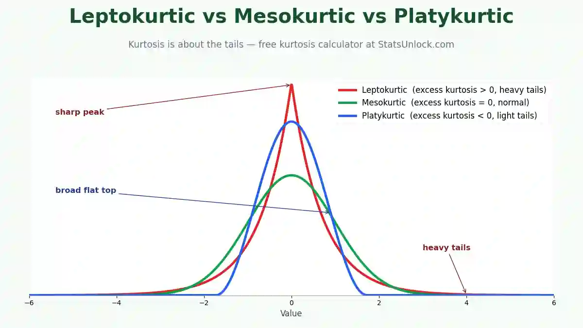
Leptokurtic: excess > 0 · Mesokurtic: excess ≈ 0 · Platykurtic: excess < 0

All three curves share the same mean and roughly the same spread — only the tail weight differs. The red leptokurtic curve has a tall, sharp center and, crucially, tails that sit above the green normal curve far from the mean: extreme values are more likely. The blue platykurtic curve is broad and flat-topped, and its tails die off below the normal curve: extreme values are rarer. The green mesokurtic bell is the normal reference in between. This is the single picture to remember when comparing leptokurtic vs mesokurtic vs platykurtic distributions.

🧭 When to Use This Tool

Use this kurtosis calculator whenever you need to check tail weight before choosing a statistical test, screen for outlier-prone variables before regression or ANOVA, describe your data in a thesis or paper, decide whether the standard deviation is a trustworthy summary of spread, assess financial or reliability data where extreme events matter most, or teach the difference between leptokurtic, platykurtic, and mesokurtic distributions. It works with any continuous or discrete numeric variable and is designed for researchers, students, data analysts, and instructors.

⚠ Assumptions & Limitations

Kurtosis assumes your data are measured on at least an interval scale and come from a single meaningful group — a mixture of two populations can fake either heavy or light tails. It is the most outlier-sensitive of all moment statistics: because deviations are raised to the fourth power, a single extreme value can dominate the entire estimate, so always inspect the plots before trusting the number. Estimates from small samples (n < 50) are very unstable, with wide standard errors; treat them as descriptive only. Excess kurtosis near zero does not prove normality — check skewness and run a Shapiro-Wilk test as well. Kurtosis has a mathematical floor of −2 (excess), so extreme platykurtosis is bounded while leptokurtosis is unbounded. Finally, different software uses different formulas (g₂ vs G₂ vs b₂) and some report raw kurtosis (normal = 3) instead of excess (normal = 0); this tool reports both g₂ and the adjusted G₂ used by SPSS, Excel, and R so your numbers match your software.

🏁 Conclusion

Kurtosis answers one question: how often should you expect extreme values? A leptokurtic distribution (excess kurtosis above 0) says "often" — its heavy tails produce outliers well beyond what a normal distribution predicts. A platykurtic distribution (excess kurtosis below 0) says "almost never" — its light tails keep every observation near the center. The normal distribution defines the neutral point: raw kurtosis 3, excess kurtosis 0, mesokurtic.

Why does this matter in practice? Because tail weight decides whether your standard deviation, confidence intervals, and variance-based tests can be trusted. In leptokurtic data a couple of tail observations inflate the SD, widen or destabilize intervals, and break variance tests — which is why finance abandoned the normal distribution for returns, and why robust statistics (median, MAD, trimmed means, bootstrapping) exist. Platykurtic data are gentler, typically making tests conservative, but strong platykurtosis is often a clue that your variable is bounded or bimodal and deserves a second look. And because kurtosis is blind to asymmetry, it must always be read together with skewness: normal-like data require both statistics near zero and a clean Q-Q plot.

This calculator gives you everything needed to make and defend that judgement: the excess kurtosis g₂ and software-matching adjusted G₂, the standard error and z-test, four diagnostic plots including a direct normal-curve overlay, and APA-style sentences ready to paste into your Results section. Run your data, look at the tails, and let the number confirm what the picture shows — that is all "leptokurtic vs platykurtic" ever asks of you.

❓ Frequently Asked Questions

What is kurtosis in simple terms?

Kurtosis measures how heavy the tails of a distribution are — how prone your data are to producing extreme values (outliers) compared with a normal distribution. High kurtosis means outliers are common; low kurtosis means they are rare.

What is the difference between leptokurtic and platykurtic?

Leptokurtic means excess kurtosis above 0 — heavier tails and more outliers than normal. Platykurtic means excess kurtosis below 0 — lighter tails and fewer outliers. Mesokurtic means excess kurtosis near 0, like the normal distribution.

What is the kurtosis of a normal distribution?

Raw kurtosis of exactly 3, which equals excess kurtosis of 0. Because most software reports excess kurtosis, a value near 0 in SPSS, Excel, or R means normal-like tail weight.

What is excess kurtosis?

Excess kurtosis is raw kurtosis minus 3. The subtraction re-centres the scale so the normal distribution scores 0, making positive values (leptokurtic) and negative values (platykurtic) instantly interpretable.

Does high kurtosis mean a more peaked distribution?

Not reliably — this is the most common kurtosis misconception. Kurtosis is driven by the fourth power of deviations, so it measures tail weight, not peak shape. A flat-topped distribution can still be leptokurtic if its tails are heavy (Westfall, 2014).

What kurtosis value is acceptable for normality?

Excess kurtosis within ±1 is commonly treated as normal-like. Many applied researchers accept ±2, and structural equation modeling literature tolerates up to ±7 with large samples (West et al., 1995). Beyond those bounds, use robust methods.

What is an example of a leptokurtic distribution?

Daily stock returns are the classic case: most days change little, but occasional crashes and rallies create heavy tails. Insurance claims, reaction times, and Student's t with low degrees of freedom are other standard examples.

What is an example of a platykurtic distribution?

The uniform distribution, with excess kurtosis of exactly −1.2. Practical examples include random lottery numbers, evenly spread bounded ratings, and any variable deliberately sampled across its whole range.

What is the difference between kurtosis and skewness?

Skewness measures asymmetry — whether one tail is longer than the other. Kurtosis measures combined tail weight — how extreme the outliers are in both tails. They are independent: a perfectly symmetric distribution can be strongly leptokurtic.

Is high kurtosis good or bad?

Neither — it is information. High kurtosis warns you that extreme events are likelier than the normal distribution suggests, which matters enormously in risk management, quality control, and any analysis that relies on the standard deviation.

Can kurtosis be negative?

Excess kurtosis can be negative down to a mathematical floor of −2 (raw kurtosis floor of 1). Raw kurtosis itself is always positive. Negative excess kurtosis simply means lighter tails than a normal distribution.

How do I fix high kurtosis in my data?

First check whether the tail values are errors or genuine. For genuine heavy tails: transform (log or square root often helps when skew accompanies kurtosis), winsorize or trim, use robust estimators (median, MAD), bootstrap your confidence intervals, or fit an explicitly heavy-tailed model such as Student's t regression.

How large should my sample be for a reliable kurtosis estimate?

Larger than for almost any other descriptive statistic. Below n = 50 the estimate is extremely noisy because single observations dominate the fourth moment; n ≥ 100 gives a usable estimate, and n ≥ 200 is preferable for formal testing.

Do SPSS, Excel, and R report the same kurtosis?

SPSS, Excel's KURT function, and R's e1071::kurtosis(type = 2) all report the adjusted excess kurtosis G₂, which is what this calculator shows — so the numbers will match. Python's scipy.stats.kurtosis default (bias = True) reports the moment coefficient g₂, which this tool also displays.

Can I use a t-test on leptokurtic data?

The t-test is fairly robust to kurtosis when samples are moderate to large (n ≥ 30 per group), because the sampling distribution of the mean normalizes. The bigger danger is to variance-based tests (F-test, Levene's) and to the SD itself — for strongly leptokurtic data, prefer Welch's t-test, rank-based tests, or bootstrapped intervals.

What does a leptokurtic box plot look like?

A relatively short box (dense middle 50%) with numerous outlier dots beyond both whiskers. A platykurtic box plot shows the opposite — a wide box with long whiskers and no outlier dots at all.

What does kurtosis look like on a Q-Q plot?

Leptokurtic data form an S-shape: points rise above the reference line at the upper end and fall below it at the lower end. Platykurtic data bend the opposite way, flattening at both extremes. Points hugging the line indicate mesokurtic tails.

What is the fourth moment and why does kurtosis use it?

The fourth moment is the average of deviations from the mean raised to the fourth power. Raising to the fourth power makes large deviations overwhelmingly dominant — a deviation twice as large contributes sixteen times as much — which is exactly why kurtosis reads the tails.

Why do skewness and kurtosis get reported together?

Together they summarize distribution shape: skewness captures asymmetry, kurtosis captures tail weight. Normality screening conventions (and tests like D'Agostino's K²) combine both, because a distribution can pass one check while badly failing the other.

Is "kurtosis" related to "curtosis" or "curtness"?

No — kurtosis comes from the Greek kyrtos, meaning curved or arched. "Curtosis" is simply a common misspelling. The prefixes tell the story: lepto- (slender), platy- (broad), meso- (middle).

📚 References

Joanes, D. N., & Gill, C. A. (1998). Comparing measures of sample skewness and kurtosis. Journal of the Royal Statistical Society: Series D (The Statistician), 47(1), 183–189. https://doi.org/10.1111/1467-9884.00122
Westfall, P. H. (2014). Kurtosis as peakedness, 1905–2014. R.I.P. The American Statistician, 68(3), 191–195. https://doi.org/10.1080/00031305.2014.917055
DeCarlo, L. T. (1997). On the meaning and use of kurtosis. Psychological Methods, 2(3), 292–307. https://doi.org/10.1037/1082-989X.2.3.292
Kim, H.-Y. (2013). Statistical notes for clinical researchers: Assessing normal distribution using skewness and kurtosis. Restorative Dentistry & Endodontics, 38(1), 52–54. https://doi.org/10.5395/rde.2013.38.1.52
Balanda, K. P., & MacGillivray, H. L. (1988). Kurtosis: A critical review. The American Statistician, 42(2), 111–119. https://doi.org/10.1080/00031305.1988.10475539
Moors, J. J. A. (1986). The meaning of kurtosis: Darlington reexamined. The American Statistician, 40(4), 283–284. https://doi.org/10.1080/00031305.1986.10475415
Blanca, M. J., Arnau, J., López-Montiel, D., Bono, R., & Bendayan, R. (2013). Skewness and kurtosis in real data samples. Methodology, 9(2), 78–84. https://doi.org/10.1027/1614-2241/a000057
Curran, P. J., West, S. G., & Finch, J. F. (1996). The robustness of test statistics to nonnormality and specification error in confirmatory factor analysis. Psychological Methods, 1(1), 16–29. https://doi.org/10.1037/1082-989X.1.1.16
West, S. G., Finch, J. F., & Curran, P. J. (1995). Structural equation models with nonnormal variables: Problems and remedies. In R. H. Hoyle (Ed.), Structural Equation Modeling: Concepts, Issues, and Applications (pp. 56–75). Sage. APA PsycNet record
D'Agostino, R. B., Belanger, A., & D'Agostino, R. B., Jr. (1990). A suggestion for using powerful and informative tests of normality. The American Statistician, 44(4), 316–321. https://doi.org/10.1080/00031305.1990.10475751
Mardia, K. V. (1970). Measures of multivariate skewness and kurtosis with applications. Biometrika, 57(3), 519–530. https://doi.org/10.1093/biomet/57.3.519
Micceri, T. (1989). The unicorn, the normal curve, and other improbable creatures. Psychological Bulletin, 105(1), 156–166. https://doi.org/10.1037/0033-2909.105.1.156
Ho, A. D., & Yu, C. C. (2015). Descriptive statistics for modern test score distributions: Skewness, kurtosis, discreteness, and ceiling effects. Educational and Psychological Measurement, 75(3), 365–388. https://doi.org/10.1177/0013164414548576
Cain, M. K., Zhang, Z., & Yuan, K.-H. (2017). Univariate and multivariate skewness and kurtosis for measuring nonnormality: Prevalence, influence and estimation. Behavior Research Methods, 49(5), 1716–1735. https://doi.org/10.3758/s13428-016-0814-1
Cont, R. (2001). Empirical properties of asset returns: Stylized facts and statistical issues. Quantitative Finance, 1(2), 223–236. https://doi.org/10.1080/713665670
Bulmer, M. G. (1979). Principles of Statistics. Dover Publications. Publisher page
Tabachnick, B. G., & Fidell, L. S. (2019). Using Multivariate Statistics (7th ed.). Pearson. Publisher page
Field, A. (2018). Discovering Statistics Using IBM SPSS Statistics (5th ed.). Sage. Publisher page
NIST/SEMATECH. (2012). Measures of skewness and kurtosis. In e-Handbook of Statistical Methods. https://www.itl.nist.gov/div898/handbook/eda/section3/eda35b.htm
Hazewinkel, M. (Ed.). (2001). Excess coefficient. In Encyclopedia of Mathematics. Springer. encyclopediaofmath.org