


Normal Distribution Calculator
Find any normal probability in seconds. Enter a mean and standard deviation, or paste your own data, and get P(X ≤ x), P(X ≥ x), the area between two values, z scores, percentiles, a Shapiro-Wilk normality check and four clear charts, with every step shown.
⚡ 0. Quick Answer
A normal distribution calculator turns a value into a probability. First convert the value to a z score, z = (x − μ) ÷ σ, then read the area under the bell curve to the left of z.
Example: leaf lengths have mean 52.44 mm and SD 4.19 mm. For x = 60, z = 1.80, so P(X ≤ 60) = 0.9643. About 96.4% of leaves are 60 mm or shorter.
Rule of thumb: 68% of values fall within 1 SD of the mean, 95% within 2 SD and 99.7% within 3 SD. The total area under a normal curve is always exactly 1.
🔑 Key Takeaways
- A normal distribution calculator needs only 2 numbers: the mean μ and the standard deviation σ.
- Every normal curve is symmetric, so the mean, median and mode are equal and exactly 50% of values lie below the mean.
- The z score tells you how many SDs a value is from the mean. z = 1.96 cuts off the top 2.5%.
- The empirical rule: 68.27% within 1 SD, 95.45% within 2 SD, 99.73% within 3 SD.
- Before you trust a normal probability for real data, check normality. A Shapiro-Wilk p > 0.05 means no clear evidence against normality.
- For a binomial count, the normal curve is a good approximation when np ≥ 5 and n(1 − p) ≥ 5, with a 0.5 continuity correction.
📚 1. What Is the Normal Distribution?
The normal distribution is a smooth, bell-shaped curve that describes how many natural measurements spread around their average. Most values sit close to the middle. Fewer values sit far away. The curve falls off the same way on both sides. It is also called the Gaussian distribution or the bell curve.
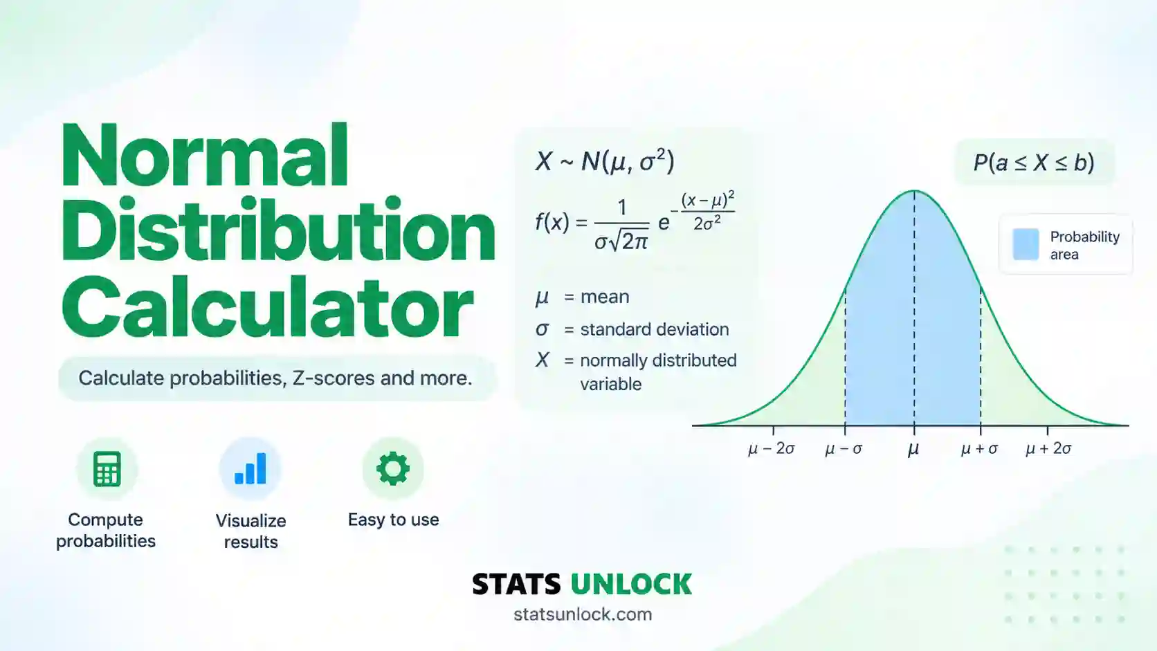
Normal distribution notation. We write X ~ N(μ, σ²). Read it as "X is normally distributed with mean μ and variance σ²". The mean sets the centre of the curve. The standard deviation σ sets its width. The special case N(0, 1) is the standard normal distribution, and its values are called z scores.
The equation of a normal distribution (its probability density function) is:
The height of this curve is not a probability. Probability is the area under the curve between two points. The total area under any normal curve is exactly 1, which is 100%.
Characteristics of a normal distribution:
- It is symmetric around the mean, so the mean, median and mode are all equal.
- It is unimodal: one single peak at μ.
- The tails never touch the x axis. They get closer forever but never reach zero.
- The inflection points, where the curve changes from bending down to bending up, are at μ − σ and μ + σ.
- Skewness is 0 and excess kurtosis is 0.
- The expected value of a normal distribution is μ, and its variance is σ².
- The sum of normal distributions is also normal. If X and Y are independent normals, X + Y ~ N(μX + μY, σ²X + σ²Y).
A worked one-liner: leaf length has μ = 52.44 mm and σ = 4.19 mm. A 60 mm leaf has z = (60 − 52.44) ÷ 4.19 = 1.80, and the area to the left of z = 1.80 is 0.9643.
Who uses it: doctors use it to set reference ranges for blood tests. Teachers use it to turn raw marks into percentiles. Engineers use it for quality control and tolerance limits. Psychologists scale IQ tests to N(100, 15²). Ecologists use it for body size and measurement error. Finance uses it (with care) for returns. Nearly every t test, ANOVA and regression assumes normal errors.
Why it is everywhere: the central limit theorem says that the mean of many independent small effects tends toward a normal distribution, whatever the shape of each effect. That is why sample means are close to normal even when raw data are not.
Related ideas. A bivariate normal distribution describes two variables that are jointly normally distributed, such as height and weight. It adds a correlation ρ to the two means and two SDs, and its contour lines are ellipses. A non normal distribution is any shape that breaks the bell: skewed, heavy tailed, bounded or with two peaks.
| Feature | Normal distribution | Standard normal distribution | Student t distribution |
|---|---|---|---|
| Notation | N(μ, σ²) | N(0, 1) | t(df) |
| Mean | μ | 0 | 0 |
| Standard deviation | σ | 1 | √(df ÷ (df − 2)) |
| Tails | Thin | Thin | Heavier, approach normal as df grows |
| Use it when | You know or estimate μ and σ | Reading a z table | σ is unknown and n is small |
🧮 2. Set Up Your Data
Type one value per cell. Each column becomes a group. Edit the column names in the top row. Empty cells are ignored.
Your probability question
📊 3. Results
🧠 4. Interpretation of Results, In Detail
4.1 Your probability, in plain words
A normal probability is a share of the whole population. P(X ≤ 60) = 0.9643 means that, if the variable really follows this normal curve, 96.43% of all values are 60 or less. It also means that one randomly chosen value has a 96.43% chance of being 60 or less. Both readings are correct. Use whichever is easier for your reader.
Always say which side of the value you mean. "The probability of 60" has no meaning for a continuous variable, because the chance of any single exact value is zero. You need "at most 60", "at least 60" or "between 45 and 60".
4.2 The z score: how unusual is this value?
The z score is the distance from the mean in standard deviation units. z = 0 is exactly average. z = 1 is one SD above the mean. z = −2 is two SDs below. A z score lets you compare values measured on different scales, such as a height in cm and a score out of 100.
| |z| | Share of values further from the mean | Plain meaning |
|---|---|---|
| below 1 | more than 31.7% | Ordinary. Most values look like this. |
| 1 to 2 | 4.6% to 31.7% | A bit high or low, still common. |
| 2 to 3 | 0.27% to 4.6% | Unusual. About 1 in 20 to 1 in 370. |
| above 3 | less than 0.27% | Very rare. Check for a data error first. |
4.3 Left tail, right tail, between and outside
These four areas are linked. Once you have one, the others follow:
- Right tail = 1 − left tail. P(X ≥ 60) = 1 − 0.9643 = 0.0357.
- Between = left tail at b minus left tail at a. P(45 ≤ X ≤ 60) = 0.9643 − 0.0381 = 0.9262.
- Outside = 1 − between = 0.0738.
For a continuous variable, ≤ and < give the same answer. P(X < 60) equals P(X ≤ 60). This is not true for counts, which is why the binomial approximation needs a continuity correction (Section 4.10).
4.4 Percentiles and the inverse normal
The inverse normal answers the reverse question: "Which value cuts off the lowest p%?" For leaf length, the 90th percentile is 57.81 mm. So 90% of leaves are shorter than 57.81 mm and 10% are longer. The formula is x = μ + zp × σ, where zp comes from the z table read backwards. Reference ranges in medicine are built this way: the central 95% runs from μ − 1.96σ to μ + 1.96σ.
4.5 The empirical rule, and what your data say about it
For a perfect normal distribution, 68.27% of values lie within 1 SD of the mean, 95.45% within 2 SD and 99.73% within 3 SD. Chart 4 compares your data with these targets. Small samples wobble. With 16 values, 62.5% in place of 68.3% is normal chance. But if far more than 68% sit within 1 SD, the curve is too peaked. If far fewer than 95% sit within 2 SD, the tails are too heavy. Both are signs of a non normal distribution.
4.6 How to tell if data is normally distributed: the Shapiro-Wilk test
The Shapiro-Wilk test asks: "Could these data come from a normal distribution?" W runs from 0 to 1. Values near 1 mean the sorted data match normal quantiles closely.
- p > α (usually 0.05): no clear evidence against normality. It does not prove the data are normal.
- p ≤ α: the data depart from normality. Look at the Q-Q plot to see how.
The test depends heavily on sample size. With 8 values it misses almost everything. With 2000 values it flags differences too small to matter. So always read the p value together with Charts 2 and 3.
4.7 Skewness and kurtosis
Skewness measures lopsidedness. 0 is symmetric. Positive means a long right tail (income, reaction time). Negative means a long left tail (easy exam scores). Excess kurtosis measures tail weight. 0 is normal. Positive means heavy tails and more outliers. Negative means light tails and a flat top.
A simple rule from Kim (2013): divide each by its standard error. For n under 50, |z| above 1.96 is a problem. For n from 50 to 300, use 3.29. For n above 300, look at the raw values: |skewness| above 2 or |excess kurtosis| above 7 is a real departure.
4.8 Reading the histogram and the Q-Q probability plot
Chart 2, the normal distribution histogram. A histogram of normal distribution data looks like a rough bell. The bars should follow the line. Count data with few values will look lumpy. That is fine. What matters is a clear lean to one side, two peaks, or a long tail.
Chart 3, the normal probability plot. Each point pairs a sorted value with the value a perfect normal would give. Points on the straight line mean the data are normally distributed. The shape of the bend tells you the problem:
| Q-Q pattern | Meaning |
|---|---|
| Points follow the line | Approximately normal |
| Curve bending upward at the right (a smile) | Right skew |
| Curve bending down at the left (a frown) | Left skew |
| S shape, ends pulling away from the line | Heavy tails (positive kurtosis) |
| Reverse S, ends flattening toward the line | Light tails (negative kurtosis) |
| One or two points far off at an end | Outliers |
| Steps or flat runs | Rounded or discrete data |
4.9 Could the graph represent a variable with a normal distribution?
This is a common exam question. Answer "yes" only if all of these hold: the graph has one peak; it is roughly symmetric about that peak; it falls off smoothly on both sides; and it does not stop abruptly at a boundary such as zero. Answer "no" if the graph is skewed, has two humps, is flat, or is cut off on one side. The mean of the normal distribution shown is always the x value under the peak.
4.10 Normal approximation to the binomial distribution
A binomial count X (successes in n trials) has mean np and SD √(np(1 − p)). When np ≥ 5 and n(1 − p) ≥ 5, its shape is close to normal. Because counts are whole numbers, widen each bar by 0.5 on each side. That is the continuity correction: P(X ≤ 25) becomes P(Y ≤ 25.5). For n = 50 and p = 0.4, the approximation gives 0.9438 and the exact binomial is 0.9427. Without the correction you would get 0.9255, which is much worse.
4.11 Decision guide
| What you see | What to do |
|---|---|
| Shapiro-Wilk p > α, straight Q-Q plot, bell-shaped histogram | Use the normal model Report the probability with μ and σ. |
| p ≤ α but n is large and the plots look close to normal | Use with care Middle probabilities are fine. Tail probabilities (beyond 2 SD) may be off. |
| Clear right skew, positive values only | Transform Try a log transform, then check again. Or use empirical percentiles. |
| Two peaks | Split the groups You probably have two populations mixed together. |
| Normal model gives a big chance of impossible values (below 0) | Do not use The normal curve does not fit a bounded variable. |
4.12 Common mistakes this calculator prevents
- Reading the wrong side of the z table. The tool always states which area it found and shades it on Chart 1.
- Using the population SD by accident. The default is the sample SD, matching R and Excel STDEV.S.
- Trusting a normal probability for skewed data. Every run checks normality, skewness and kurtosis, and warns you.
- Forgetting the continuity correction for binomial counts. It is applied and shown.
- Treating "not significant" as proof of normality. The wording in Section 5 avoids that claim.
- Mixing up a negative z value with a negative probability. Probabilities are always between 0 and 1.
✍ 5. How to Write Your Results in Research
A good write-up of a normal distribution result always has four parts: (1) the variable and its units, (2) the model, N(μ, σ²), with n if the parameters came from data, (3) the probability or percentile with the exact question, and (4) evidence that the normal model fits. Leave out part 4 and a reviewer will ask for it.
📌 Key conventions for this style
- Italicise statistical symbols: M, SD, W, p, z, n.
- Report exact p values to two or three decimals; write p < .001 for very small values.
- APA drops the leading zero for values that cannot exceed 1, such as p and probabilities (p = .954).
- Say "approximately normal" or "no evidence against normality", never "the data are normal".
📌 Key conventions for this style
- Name every normality check you used, both formal tests and plots.
- State the significance level before the result.
- Say whether the SD used n or n − 1.
- If the check fails, say what you did next: transform, trim or switch method.
- Put the Q-Q plot in an appendix if the main text is short on space.
📌 Key conventions for this style
- Turn probabilities into "out of 100" frequencies. People understand 4 in 100 better than 0.0357.
- No symbols, no z, no p.
- Give units every time a number appears.
- Say "about" because the normal model is an approximation.
📌 Key conventions for this style
- One line each for Methods, Results and Conclusion.
- Lead the Results line with the headline probability.
- Use a percentage in the Conclusion for a lay audience.
- Keep decimal places the same throughout the poster.
📌 Key conventions for this style
- Give every setting another person needs to repeat the result: SD type, α, question type and cut-off values.
- Name the normality test and the software.
- Pre-register your plan for a failed normality check before you see the data.
- Share the raw data or at least n, mean and SD to four decimals.
5.1 Phrases to use, and phrases to avoid
| Write this | Not this | Why |
|---|---|---|
| "approximately normally distributed" | "normally distributed" (as a proven fact) | A test can only fail to find a departure. |
| "no evidence of departure from normality, W = .98, p = .954" | "normality was confirmed" | A large p value is not confirmation. |
| "the expected proportion below 60 mm is 96.4%" | "96.4% of leaves are below 60 mm" | The first is a model prediction; the second claims an observed count. |
| "P(X ≥ 130) = .023" | "the probability of 130 is .023" | A single exact value has probability zero. |
| "z = 1.80" | "z = 1.8029" in running text | Two decimals is enough for z in prose. |
5.2 What to put in a table
For several groups, give one row per group with columns n, M, SD, W, p (Shapiro-Wilk) and the probability you computed. Add a note under the table: "Probabilities assume a normal distribution with the sample mean and SD; SD uses n − 1."
∑ 6. Formulas Used
🔀 7. Normal Distribution Calculation Flowchart, Step by Step
This flowchart shows how a normal distribution probability is calculated, step by step, from raw data to a checked answer. Every box uses the same worked example as the Excel, R and Python sections: 16 leaf lengths in mm, and the question "what share of leaves are 60 mm or shorter?"
Check any box yourself: the Excel sheet in Section 9, the R script in Section 10 and the Python script in Section 11 all return a mean of 52.4375, an SD of 4.1947, z = 1.8029 and P(X ≤ 60) = 0.9643.
📝 8. How to Use This Calculator
- Enter your data. The default box takes comma-separated numbers, as the placeholder shows:
52, 48, 55, 61, 47, .... Spaces, tabs, semicolons and new lines also work, so a column pasted from Excel is fine. - Name each group. The name field above each box is editable. Type something like Site A and it appears in the table, the charts and the report.
- Add groups to compare. Press Add group. Each group gets its own mean, SD, normal curve and normality test.
- Or upload a file. On the Upload tab, choose a CSV or Excel file and click the column names you want. Each column you click becomes its own group.
- Or skip the data. For a textbook question, set "Where do μ and σ come from?" to "I will type μ and σ myself". Use μ = 0 and σ = 1 for the standard normal distribution.
- Pick your question. Left tail, right tail, between, outside, percentile, central interval or the binomial approximation.
- Type the values. For example x = 60, or a = 45 and b = 60, or p = 90 for the 90th percentile.
- Press Calculate Normal Distribution. Nothing is computed until you do. Changing any input clears old results so you never read stale numbers.
- Read the answer and the checks. The top box gives the probability. The assumption table tells you whether the normal model fits your data.
- Use the charts and export. Chart 1 shows the shaded area. Section 5 fills in five report styles. Download the text report or a print-ready PDF.
📈 9. How to Calculate Normal Distribution in Excel
Excel has built-in functions for every normal distribution calculation: the left-tail probability, the density, the inverse and the z score. What trips people up is the TRUE or FALSE last argument, the right tail, and the fact that Excel has no Shapiro-Wilk test.
=NORM.DIST(60, AVERAGE(A2:A17), STDEV.S(A2:A17), TRUE). That is P(X ≤ 60), here 0.9643.9.1 The functions you need
| You want | Excel function | Note |
|---|---|---|
| P(X ≤ x), left tail | =NORM.DIST(x, mean, sd, TRUE) | TRUE means cumulative area |
| Curve height f(x) | =NORM.DIST(x, mean, sd, FALSE) | FALSE gives the density, not a probability |
| P(X ≥ x), right tail | =1-NORM.DIST(x, mean, sd, TRUE) | There is no right-tail function |
| P(a ≤ X ≤ b) | =NORM.DIST(b,m,s,TRUE)-NORM.DIST(a,m,s,TRUE) | Upper minus lower |
| z table value Φ(z) | =NORM.S.DIST(z, TRUE) | Standard normal N(0, 1) |
| x for a percentile | =NORM.INV(p, mean, sd) | Inverse normal |
| z for a percentile | =NORM.S.INV(p) | =NORM.S.INV(0.975) gives 1.96 |
| z score | =STANDARDIZE(x, mean, sd) | Same as (x − mean) ÷ sd |
| Skewness, excess kurtosis | =SKEW(rng), =KURT(rng) | Bias-corrected, like this page |
=NORM.DIST(60, 52.44, 4.19, FALSE) returns 0.0187. That is the height of the curve, not a probability. Almost every wrong answer posted online comes from this. For areas, always use TRUE.9.2 Step by step
1 Put your numbers in one column
Paste the values down column A with a label in row 1. The 16 leaf lengths fill A2:A17.
The first eight of the 16 leaf lengths in A2:A17, with the header in A1.
2 Estimate the mean and standard deviation
=AVERAGE(A2:A17)=STDEV.S(A2:A17)=COUNT(A2:A17)Put these in D2, D3 and D4 so later formulas can point at them.
Mean 52.4375, SD 4.1947, n 16. These are μ and σ for every formula that follows.
3 Convert x to a z score
=STANDARDIZE(60,D2,D3)This tells you 60 mm is 1.80 SD above the mean.
z = 1.8029 for x = 60. Look up 1.80 in the z table in Section 12 and you get 0.9641; the exact value is 0.9643.
4 Get the left, right and between probabilities
=NORM.DIST(60,D2,D3,TRUE)=1-NORM.DIST(60,D2,D3,TRUE)=NORM.DIST(60,D2,D3,TRUE)-NORM.DIST(45,D2,D3,TRUE)P(X ≤ 60) = 0.9643, P(X ≥ 60) = 0.0357, P(45 ≤ X ≤ 60) = 0.9262. The left and right tails add to exactly 1.
5 Go backwards: percentiles and critical values
=NORM.INV(0.9,D2,D3)=NORM.S.INV(0.975)=NORM.DIST(60,D2,D3,FALSE)90th percentile 57.8133 mm, critical z 1.9600, and the curve height at 60, 0.0187, which is not a probability.
9.3 The awkward cases
- No Shapiro-Wilk in Excel. Neither the functions nor the Analysis ToolPak include it. Use this calculator, R or Python for the test, and use
SKEWandKURTin Excel as a rough check (here 0.3853 and −0.4360). - Normal probability plot in Excel. Sort the data in column A. In B2 type
=NORM.S.INV((ROW()-1-0.375)/(COUNT($A$2:$A$17)+0.25))and fill down. Insert a scatter chart of B (x axis) against A (y axis). Points on a straight line mean normal data. - Histogram with a normal curve. The Analysis ToolPak Histogram tool (File → Options → Add-ins → Excel Add-ins → tick Analysis ToolPak) makes the bars. Add a second series of
=NORM.DIST(bin_mid,m,s,FALSE)*n*bin_widthand change it to a line. - Normal approximation to the binomial.
=NORM.DIST(25.5, 50*0.4, SQRT(50*0.4*0.6), TRUE)gives 0.9438. Compare with the exact=BINOM.DIST(25,50,0.4,TRUE), 0.9427. - Old function names.
NORMDIST,NORMSDIST,NORMINVandNORMSINVstill work but are kept only for compatibility. Use the dotted versions.
9.4 Why your Excel answer might differ from R or Python
| Situation | What happens | Fix |
|---|---|---|
Used STDEV.P | SD is 4.0615 instead of 4.1947, so every probability shifts | Use STDEV.S; it matches R sd() |
Python np.std(x) | NumPy defaults to the population SD, ddof = 0 | Use np.std(x, ddof=1) or x.std(ddof=1) |
| Rounded μ and σ typed by hand | 52.44 and 4.19 give 0.9644, not 0.9643 | Point at the cells instead of retyping |
| Read a printed z table | z rounded to 1.80 gives 0.9641 | Use NORM.S.DIST(z,TRUE) for full precision |
| Skewness differs from Python | SciPy skew() defaults to the biased version | Use stats.skew(x, bias=False) to match Excel SKEW |
| Kurtosis differs from R packages | Some report raw kurtosis (normal = 3), others excess (normal = 0) | Excel KURT and this page report excess kurtosis |
| Tool | P(X ≤ x) | Inverse | Density |
|---|---|---|---|
| Excel | =NORM.DIST(x,m,s,TRUE) | =NORM.INV(p,m,s) | =NORM.DIST(x,m,s,FALSE) |
| Google Sheets | =NORM.DIST(x,m,s,TRUE) | =NORM.INV(p,m,s) | =NORM.DIST(x,m,s,FALSE) |
| R | pnorm(x, m, s) | qnorm(p, m, s) | dnorm(x, m, s) |
| Python SciPy | norm.cdf(x, m, s) | norm.ppf(p, m, s) | norm.pdf(x, m, s) |
| TI-84 | normalcdf(-1E99, x, m, s) | invNorm(p, m, s) | normalpdf(x, m, s) |
9.5 Drawing a normal distribution curve in Excel
- In column F, make x values from μ − 4σ to μ + 4σ in small steps, for example
=$D$2-4*$D$3+(ROW()-2)*$D$3/10, filled down 81 rows. - In G2 type
=NORM.DIST(F2,$D$2,$D$3,FALSE)and fill down. - Select F and G, then Insert → Charts → Scatter with Smooth Lines.
- To shade P(X ≤ 60), add column H:
=IF(F2<=60,G2,NA()), add it as a series and change it to an Area chart. - Label the axes with the variable name and units. Chart 1 on this page draws the same figure automatically.
9.6 Excel errors you will probably hit
| Excel shows | Why | Fix |
|---|---|---|
#NUM! from NORM.DIST | The SD is zero or negative | Check the SD cell; all values may be identical |
#NUM! from NORM.INV | p is 0, 1, or outside 0 to 1 | Type 0.9, not 90 |
#VALUE! | Text in an argument, such as "60 mm" | Keep units in a separate column |
#DIV/0! in STANDARDIZE | SD cell is empty | Fill in D3 first |
| Probability above 1 | Used FALSE, which returns a density | Change the last argument to TRUE |
#NAME? | Typo, or an old Excel without NORM.DIST | Check spelling or use NORMDIST in Excel 2007 |
📈 10. How to Calculate Normal Distribution in R
R has four normal functions built in: pnorm for probabilities, qnorm for percentiles, dnorm for the curve height and rnorm for random values. The script below estimates μ and σ, finds every probability, runs the Shapiro-Wilk test, prints a plain-English verdict and saves one figure at 300 dpi. It uses base R only.
Rscript. Change only the x <- c(...) line and the question values.10.1 The complete script
R, base only, saves normal_distribution_plot.png
# ============================================================
# Normal distribution calculator in R
# StatsUnlock - https://statsunlock.com/normal-distribution-calculator/
# Base R only. No packages to install.
# ============================================================

# ---- 1. Your data ------------------------------------------
# Replace with your own values, or read a CSV:
#   x <- read.csv("data.csv")$column_name
x <- c(52, 48, 55, 61, 47, 50, 58, 53,
       49, 56, 51, 54, 46, 57, 50, 52)
x <- x[!is.na(x)]                 # drop missing values

label   <- "Leaf length"
units   <- "mm"
x_value <- 60                     # P(X <= x_value)
a <- 45; b <- 60                  # P(a <= X <= b)
pct <- 0.90                       # percentile to find

# ---- 2. Estimate mu and sigma ------------------------------
n     <- length(x)
mu    <- mean(x)
sigma <- sd(x)                    # n - 1, same as Excel STDEV.S

# ---- 3. Probabilities --------------------------------------
z         <- (x_value - mu) / sigma
p_left    <- pnorm(x_value, mean = mu, sd = sigma)
p_right   <- pnorm(x_value, mean = mu, sd = sigma, lower.tail = FALSE)
p_between <- pnorm(b, mu, sigma) - pnorm(a, mu, sigma)
x_pct     <- qnorm(pct, mean = mu, sd = sigma)

# ---- 4. Normality check ------------------------------------
sw <- shapiro.test(x)
d  <- x - mu
g1 <- mean(d^3) / mean(d^2)^1.5
g2 <- mean(d^4) / mean(d^2)^2 - 3
skew <- g1 * sqrt(n * (n - 1)) / (n - 2)                     # same as Excel SKEW
kurt <- ((n + 1) * g2 + 6) * (n - 1) / ((n - 2) * (n - 3))   # same as Excel KURT

# ---- 5. Print a plain-English report -----------------------
cat(sprintf("n = %d, mean = %.4f, SD = %.4f\n", n, mu, sigma))
cat(sprintf("z for x = %g: %.4f\n", x_value, z))
cat(sprintf("P(X <= %g) = %.4f\n", x_value, p_left))
cat(sprintf("P(X >= %g) = %.4f\n", x_value, p_right))
cat(sprintf("P(%g <= X <= %g) = %.4f\n", a, b, p_between))
cat(sprintf("%.0fth percentile = %.4f %s\n", pct * 100, x_pct, units))
cat(sprintf("Shapiro-Wilk W = %.4f, p = %.4f\n", sw$statistic, sw$p.value))
cat(sprintf("Skewness = %.4f, excess kurtosis = %.4f\n", skew, kurt))
if (sw$p.value > 0.05) {
  cat("Verdict: no evidence against normality, so the normal model is reasonable.\n")
  cat(sprintf("About %.1f%% of values are expected to be %g %s or less.\n",
              p_left * 100, x_value, units))
} else {
  cat("Verdict: the data depart from normality. Treat normal probabilities with caution.\n")
}

# ---- 6. One figure: histogram + normal curve + shaded area -
set.seed(1)                       # nothing random here, but seeded for habit
png("normal_distribution_plot.png", width = 7, height = 4.5, units = "in", res = 300)
xs <- seq(mu - 4 * sigma, mu + 4 * sigma, length.out = 400)
hist(x, freq = FALSE, col = "#bfdbfe", border = "#1e40af",
     xlim = range(xs), ylim = c(0, dnorm(mu, mu, sigma) * 1.15),
     main = sprintf("N(%.2f, %.2f^2), Shapiro-Wilk p = %.3f", mu, sigma, sw$p.value),
     xlab = sprintf("%s (%s)", label, units), ylab = "Density")
left <- xs[xs <= x_value]
polygon(c(min(left), left, max(left)), c(0, dnorm(left, mu, sigma), 0),
        col = adjustcolor("#16a34a", alpha.f = 0.3), border = NA)
lines(xs, dnorm(xs, mu, sigma), col = "#1d4ed8", lwd = 2)
abline(v = x_value, lty = 2, col = "#16a34a")
legend("topright", bty = "n",
       legend = c("Normal curve", sprintf("P(X <= %g) = %.4f", x_value, p_left)),
       col = c("#1d4ed8", "#16a34a"), lwd = c(2, 8))
dev.off()
cat("Saved normal_distribution_plot.png\n")
Printed output:
n = 16, mean = 52.4375, SD = 4.1947
z for x = 60: 1.8029
P(X <= 60) = 0.9643
P(X >= 60) = 0.0357
P(45 <= X <= 60) = 0.9262
90th percentile = 57.8133 mm
Shapiro-Wilk W = 0.9789, p = 0.9541
Skewness = 0.3853, excess kurtosis = -0.4360
Verdict: no evidence against normality, so the normal model is reasonable.
About 96.4% of values are expected to be 60 mm or less.
10.2 What each line does
| Line or function | What it does, and why it is there |
|---|---|
| x[!is.na(x)] | Drops missing values. mean() and sd() return NA if even one value is missing. |
| sd(x) | Sample SD with n − 1. Matches Excel STDEV.S and this page's default. |
| pnorm(x, mean, sd) | Area to the left of x. Add lower.tail = FALSE for the right tail. |
| qnorm(p, mean, sd) | Inverse normal. qnorm(0.975) gives the famous 1.959964. |
| dnorm(x, mean, sd) | Curve height, used here only to draw the bell curve. |
| shapiro.test(x) | Shapiro-Wilk test, Royston's version. Needs 3 to 5000 values. |
| skew, kurt | Bias-corrected skewness and excess kurtosis, the same formulas as Excel SKEW and KURT. |
| png(..., res = 300) | Opens a 300 dpi image file. dev.off() closes and saves it. |
| polygon() | Shades the area under the curve to the left of x_value. |
10.3 What the figure shows
The saved figure has the histogram of your data (blue bars), the fitted normal curve (dark blue line) and the shaded area for P(X ≤ 60) (green). The title carries the model and the Shapiro-Wilk p value, so the figure stands on its own in a report. If the bars follow the curve, the normal model is a fair description.
10.4 Problems and fixes
| Problem | Fix |
|---|---|
sample size must be between 3 and 5000 | Shapiro-Wilk limit. For bigger data use a Q-Q plot, or test a random sample of 5000. |
| Result is NA | Missing values. Keep the x[!is.na(x)] line. |
| Probability looks wrong | Check argument order: pnorm(q, mean, sd), and that sd is not the variance. |
| Right tail is tiny and prints 0 | Use pnorm(..., lower.tail = FALSE) or format(p, scientific = TRUE). |
| No plot file appears | You forgot dev.off(), or the working folder is not where you expect. Run getwd(). |
10.5 One-liners
pnorm(1.96)                         # 0.9750, z table value
pnorm(-1.96)                        # 0.0250, negative z table
qnorm(0.95)                         # 1.6449, one-tailed 5% critical z
pnorm(130, 100, 15, lower.tail = FALSE)   # 0.0228, IQ above 130
pnorm(25.5, 20, sqrt(12))           # 0.9438, binomial approximation
qqnorm(x); qqline(x)                # normal probability plot
📈 11. How to Calculate Normal Distribution in Python
In Python, scipy.stats.norm does the work. cdf gives left-tail probabilities, sf gives right tails, ppf gives percentiles and pdf gives the curve height. The script below mirrors the R script line for line and gives the same numbers.
Install once with pip install numpy scipy matplotlib.
11.1 The complete script
Python 3, saves normal_distribution_plot.png
# ============================================================
# Normal distribution calculator in Python
# StatsUnlock - https://statsunlock.com/normal-distribution-calculator/
# Needs: numpy, scipy, matplotlib
# ============================================================
import numpy as np
from scipy import stats
import matplotlib
matplotlib.use("Agg")            # draw without a screen
import matplotlib.pyplot as plt

# ---- 1. Your data ------------------------------------------
# Replace with your own values, or read a CSV:
#   import pandas as pd
#   x = pd.read_csv("data.csv")["column_name"].dropna().to_numpy()
x = np.array([52, 48, 55, 61, 47, 50, 58, 53,
              49, 56, 51, 54, 46, 57, 50, 52], dtype=float)
x = x[~np.isnan(x)]              # drop missing values

label = "Leaf length"
units = "mm"
x_value = 60                     # P(X <= x_value)
a, b = 45, 60                    # P(a <= X <= b)
pct = 0.90                       # percentile to find

# ---- 2. Estimate mu and sigma ------------------------------
n = len(x)
mu = x.mean()
sigma = x.std(ddof=1)            # ddof=1 matches R sd() and Excel STDEV.S

# ---- 3. Probabilities --------------------------------------
z = (x_value - mu) / sigma
p_left = stats.norm.cdf(x_value, loc=mu, scale=sigma)
p_right = stats.norm.sf(x_value, loc=mu, scale=sigma)
p_between = stats.norm.cdf(b, mu, sigma) - stats.norm.cdf(a, mu, sigma)
x_pct = stats.norm.ppf(pct, mu, sigma)

# ---- 4. Normality check ------------------------------------
w, p_sw = stats.shapiro(x)
skew = stats.skew(x, bias=False)
kurt = stats.kurtosis(x, bias=False)     # excess kurtosis

# ---- 5. Print a plain-English report -----------------------
print(f"n = {n}, mean = {mu:.4f}, SD = {sigma:.4f}")
print(f"z for x = {x_value}: {z:.4f}")
print(f"P(X <= {x_value}) = {p_left:.4f}")
print(f"P(X >= {x_value}) = {p_right:.4f}")
print(f"P({a} <= X <= {b}) = {p_between:.4f}")
print(f"{pct*100:.0f}th percentile = {x_pct:.4f} {units}")
print(f"Shapiro-Wilk W = {w:.4f}, p = {p_sw:.4f}")
print(f"Skewness = {skew:.4f}, excess kurtosis = {kurt:.4f}")
if p_sw > 0.05:
    print(f"Verdict: no evidence against normality, so the normal model is reasonable.")
    print(f"About {p_left*100:.1f}% of values are expected to be {x_value} {units} or less.")
else:
    print("Verdict: the data depart from normality. Treat normal probabilities with caution.")

# ---- 6. One figure: histogram + normal curve + shaded area -
np.random.seed(1)                # nothing random here, but seeded for habit
fig, ax = plt.subplots(figsize=(7, 4.5))
ax.hist(x, bins="sturges", density=True, color="#bfdbfe", edgecolor="#1e40af", label="Data")
grid = np.linspace(mu - 4 * sigma, mu + 4 * sigma, 400)
ax.plot(grid, stats.norm.pdf(grid, mu, sigma), color="#1d4ed8", lw=2, label="Normal curve")
fill = grid[grid <= x_value]
ax.fill_between(fill, stats.norm.pdf(fill, mu, sigma), color="#16a34a", alpha=0.3,
                label=f"P(X <= {x_value}) = {p_left:.4f}")
ax.axvline(x_value, color="#16a34a", ls="--")
ax.set_xlabel(f"{label} ({units})")
ax.set_ylabel("Density")
ax.set_title(f"N({mu:.2f}, {sigma:.2f}^2), Shapiro-Wilk p = {p_sw:.3f}")
ax.legend(frameon=False)
fig.tight_layout()
fig.savefig("normal_distribution_plot.png", dpi=300)
print("Saved normal_distribution_plot.png")
Printed output: identical to the R output in Section 10.1, ending with Saved normal_distribution_plot.png.
11.2 What each line does
| Line or function | What it does, and why it is there |
|---|---|
| x[~np.isnan(x)] | Drops missing values, which would otherwise turn every result into nan. |
| x.std(ddof=1) | Sample SD. Without ddof=1 NumPy divides by n and disagrees with R and Excel. |
| stats.norm.cdf(x, loc, scale) | Left-tail probability. loc is μ, scale is σ. |
| stats.norm.sf(x, loc, scale) | Right tail, 1 − cdf, but accurate even for tiny tails. |
| stats.norm.ppf(p, loc, scale) | Inverse normal, the percentile. |
| stats.shapiro(x) | Shapiro-Wilk W and p. Same algorithm as R. |
| bias=False | Bias-corrected skewness and kurtosis, matching Excel SKEW and KURT. |
| fig.savefig(..., dpi=300) | Saves the figure at print quality. |
11.3 What the figure shows
The same three layers as the R figure: histogram, fitted normal curve and the shaded probability. matplotlib.use("Agg") lets the script run on a server or in a terminal with no screen.
11.4 Problems and fixes
| Problem | Fix |
|---|---|
ModuleNotFoundError: scipy | Run pip install scipy in the same environment as your editor. |
| SD disagrees with Excel | Add ddof=1. |
| Warning: p-value may not be accurate for N > 5000 | Use a Q-Q plot for very large samples. |
| Skewness disagrees with Excel | Add bias=False. |
| Result is nan | Missing values remain. Keep the isnan line, or use .dropna() in pandas. |
11.5 One-liners
from scipy import stats
from scipy.stats import norm
norm.cdf(1.96)                  # 0.9750, z table value
norm.cdf(-1.96)                 # 0.0250, negative z table
norm.ppf(0.95)                  # 1.6449, one-tailed 5% critical z
norm.sf(130, 100, 15)           # 0.0228, IQ above 130
norm.cdf(25.5, 20, 12 ** 0.5)   # 0.9438, binomial approximation
stats.probplot(x, plot=plt)     # normal probability plot
📋 12. Reference Tables
12.1 Standard normal distribution table, negative z values (z table, left tail)
Each cell is Φ(z), the area to the left of z. Read the row for the first decimal and the column for the second. Example: z = −1.80 is row −1.8, column 0.00, giving 0.0359.
| z | 0.00 | 0.01 | 0.02 | 0.03 | 0.04 | 0.05 | 0.06 | 0.07 | 0.08 | 0.09 |
|---|---|---|---|---|---|---|---|---|---|---|
| −3.4 | 0.0003 | 0.0003 | 0.0003 | 0.0003 | 0.0003 | 0.0003 | 0.0003 | 0.0003 | 0.0003 | 0.0002 |
| −3.3 | 0.0005 | 0.0005 | 0.0005 | 0.0004 | 0.0004 | 0.0004 | 0.0004 | 0.0004 | 0.0004 | 0.0003 |
| −3.2 | 0.0007 | 0.0007 | 0.0006 | 0.0006 | 0.0006 | 0.0006 | 0.0006 | 0.0005 | 0.0005 | 0.0005 |
| −3.1 | 0.0010 | 0.0009 | 0.0009 | 0.0009 | 0.0008 | 0.0008 | 0.0008 | 0.0008 | 0.0007 | 0.0007 |
| −3.0 | 0.0013 | 0.0013 | 0.0013 | 0.0012 | 0.0012 | 0.0011 | 0.0011 | 0.0011 | 0.0010 | 0.0010 |
| −2.9 | 0.0019 | 0.0018 | 0.0018 | 0.0017 | 0.0016 | 0.0016 | 0.0015 | 0.0015 | 0.0014 | 0.0014 |
| −2.8 | 0.0026 | 0.0025 | 0.0024 | 0.0023 | 0.0023 | 0.0022 | 0.0021 | 0.0021 | 0.0020 | 0.0019 |
| −2.7 | 0.0035 | 0.0034 | 0.0033 | 0.0032 | 0.0031 | 0.0030 | 0.0029 | 0.0028 | 0.0027 | 0.0026 |
| −2.6 | 0.0047 | 0.0045 | 0.0044 | 0.0043 | 0.0041 | 0.0040 | 0.0039 | 0.0038 | 0.0037 | 0.0036 |
| −2.5 | 0.0062 | 0.0060 | 0.0059 | 0.0057 | 0.0055 | 0.0054 | 0.0052 | 0.0051 | 0.0049 | 0.0048 |
| −2.4 | 0.0082 | 0.0080 | 0.0078 | 0.0075 | 0.0073 | 0.0071 | 0.0069 | 0.0068 | 0.0066 | 0.0064 |
| −2.3 | 0.0107 | 0.0104 | 0.0102 | 0.0099 | 0.0096 | 0.0094 | 0.0091 | 0.0089 | 0.0087 | 0.0084 |
| −2.2 | 0.0139 | 0.0136 | 0.0132 | 0.0129 | 0.0125 | 0.0122 | 0.0119 | 0.0116 | 0.0113 | 0.0110 |
| −2.1 | 0.0179 | 0.0174 | 0.0170 | 0.0166 | 0.0162 | 0.0158 | 0.0154 | 0.0150 | 0.0146 | 0.0143 |
| −2.0 | 0.0228 | 0.0222 | 0.0217 | 0.0212 | 0.0207 | 0.0202 | 0.0197 | 0.0192 | 0.0188 | 0.0183 |
| −1.9 | 0.0287 | 0.0281 | 0.0274 | 0.0268 | 0.0262 | 0.0256 | 0.0250 | 0.0244 | 0.0239 | 0.0233 |
| −1.8 | 0.0359 | 0.0351 | 0.0344 | 0.0336 | 0.0329 | 0.0322 | 0.0314 | 0.0307 | 0.0301 | 0.0294 |
| −1.7 | 0.0446 | 0.0436 | 0.0427 | 0.0418 | 0.0409 | 0.0401 | 0.0392 | 0.0384 | 0.0375 | 0.0367 |
| −1.6 | 0.0548 | 0.0537 | 0.0526 | 0.0516 | 0.0505 | 0.0495 | 0.0485 | 0.0475 | 0.0465 | 0.0455 |
| −1.5 | 0.0668 | 0.0655 | 0.0643 | 0.0630 | 0.0618 | 0.0606 | 0.0594 | 0.0582 | 0.0571 | 0.0559 |
| −1.4 | 0.0808 | 0.0793 | 0.0778 | 0.0764 | 0.0749 | 0.0735 | 0.0721 | 0.0708 | 0.0694 | 0.0681 |
| −1.3 | 0.0968 | 0.0951 | 0.0934 | 0.0918 | 0.0901 | 0.0885 | 0.0869 | 0.0853 | 0.0838 | 0.0823 |
| −1.2 | 0.1151 | 0.1131 | 0.1112 | 0.1093 | 0.1075 | 0.1056 | 0.1038 | 0.1020 | 0.1003 | 0.0985 |
| −1.1 | 0.1357 | 0.1335 | 0.1314 | 0.1292 | 0.1271 | 0.1251 | 0.1230 | 0.1210 | 0.1190 | 0.1170 |
| −1.0 | 0.1587 | 0.1562 | 0.1539 | 0.1515 | 0.1492 | 0.1469 | 0.1446 | 0.1423 | 0.1401 | 0.1379 |
| −0.9 | 0.1841 | 0.1814 | 0.1788 | 0.1762 | 0.1736 | 0.1711 | 0.1685 | 0.1660 | 0.1635 | 0.1611 |
| −0.8 | 0.2119 | 0.2090 | 0.2061 | 0.2033 | 0.2005 | 0.1977 | 0.1949 | 0.1922 | 0.1894 | 0.1867 |
| −0.7 | 0.2420 | 0.2389 | 0.2358 | 0.2327 | 0.2296 | 0.2266 | 0.2236 | 0.2206 | 0.2177 | 0.2148 |
| −0.6 | 0.2743 | 0.2709 | 0.2676 | 0.2643 | 0.2611 | 0.2578 | 0.2546 | 0.2514 | 0.2483 | 0.2451 |
| −0.5 | 0.3085 | 0.3050 | 0.3015 | 0.2981 | 0.2946 | 0.2912 | 0.2877 | 0.2843 | 0.2810 | 0.2776 |
| −0.4 | 0.3446 | 0.3409 | 0.3372 | 0.3336 | 0.3300 | 0.3264 | 0.3228 | 0.3192 | 0.3156 | 0.3121 |
| −0.3 | 0.3821 | 0.3783 | 0.3745 | 0.3707 | 0.3669 | 0.3632 | 0.3594 | 0.3557 | 0.3520 | 0.3483 |
| −0.2 | 0.4207 | 0.4168 | 0.4129 | 0.4090 | 0.4052 | 0.4013 | 0.3974 | 0.3936 | 0.3897 | 0.3859 |
| −0.1 | 0.4602 | 0.4562 | 0.4522 | 0.4483 | 0.4443 | 0.4404 | 0.4364 | 0.4325 | 0.4286 | 0.4247 |
| −0.0 | 0.5000 | 0.4960 | 0.4920 | 0.4880 | 0.4840 | 0.4801 | 0.4761 | 0.4721 | 0.4681 | 0.4641 |
Conclusion: every value in the negative normal distribution table is below 0.5, because negative z values lie left of the mean.
12.2 Standard normal distribution table, positive z values
Example: z = 1.80 is row 1.8, column 0.00, giving 0.9641. For z = 1.96, row 1.9 and column 0.06 give 0.9750.
| z | 0.00 | 0.01 | 0.02 | 0.03 | 0.04 | 0.05 | 0.06 | 0.07 | 0.08 | 0.09 |
|---|---|---|---|---|---|---|---|---|---|---|
| 0.0 | 0.5000 | 0.5040 | 0.5080 | 0.5120 | 0.5160 | 0.5199 | 0.5239 | 0.5279 | 0.5319 | 0.5359 |
| 0.1 | 0.5398 | 0.5438 | 0.5478 | 0.5517 | 0.5557 | 0.5596 | 0.5636 | 0.5675 | 0.5714 | 0.5753 |
| 0.2 | 0.5793 | 0.5832 | 0.5871 | 0.5910 | 0.5948 | 0.5987 | 0.6026 | 0.6064 | 0.6103 | 0.6141 |
| 0.3 | 0.6179 | 0.6217 | 0.6255 | 0.6293 | 0.6331 | 0.6368 | 0.6406 | 0.6443 | 0.6480 | 0.6517 |
| 0.4 | 0.6554 | 0.6591 | 0.6628 | 0.6664 | 0.6700 | 0.6736 | 0.6772 | 0.6808 | 0.6844 | 0.6879 |
| 0.5 | 0.6915 | 0.6950 | 0.6985 | 0.7019 | 0.7054 | 0.7088 | 0.7123 | 0.7157 | 0.7190 | 0.7224 |
| 0.6 | 0.7257 | 0.7291 | 0.7324 | 0.7357 | 0.7389 | 0.7422 | 0.7454 | 0.7486 | 0.7517 | 0.7549 |
| 0.7 | 0.7580 | 0.7611 | 0.7642 | 0.7673 | 0.7704 | 0.7734 | 0.7764 | 0.7794 | 0.7823 | 0.7852 |
| 0.8 | 0.7881 | 0.7910 | 0.7939 | 0.7967 | 0.7995 | 0.8023 | 0.8051 | 0.8078 | 0.8106 | 0.8133 |
| 0.9 | 0.8159 | 0.8186 | 0.8212 | 0.8238 | 0.8264 | 0.8289 | 0.8315 | 0.8340 | 0.8365 | 0.8389 |
| 1.0 | 0.8413 | 0.8438 | 0.8461 | 0.8485 | 0.8508 | 0.8531 | 0.8554 | 0.8577 | 0.8599 | 0.8621 |
| 1.1 | 0.8643 | 0.8665 | 0.8686 | 0.8708 | 0.8729 | 0.8749 | 0.8770 | 0.8790 | 0.8810 | 0.8830 |
| 1.2 | 0.8849 | 0.8869 | 0.8888 | 0.8907 | 0.8925 | 0.8944 | 0.8962 | 0.8980 | 0.8997 | 0.9015 |
| 1.3 | 0.9032 | 0.9049 | 0.9066 | 0.9082 | 0.9099 | 0.9115 | 0.9131 | 0.9147 | 0.9162 | 0.9177 |
| 1.4 | 0.9192 | 0.9207 | 0.9222 | 0.9236 | 0.9251 | 0.9265 | 0.9279 | 0.9292 | 0.9306 | 0.9319 |
| 1.5 | 0.9332 | 0.9345 | 0.9357 | 0.9370 | 0.9382 | 0.9394 | 0.9406 | 0.9418 | 0.9429 | 0.9441 |
| 1.6 | 0.9452 | 0.9463 | 0.9474 | 0.9484 | 0.9495 | 0.9505 | 0.9515 | 0.9525 | 0.9535 | 0.9545 |
| 1.7 | 0.9554 | 0.9564 | 0.9573 | 0.9582 | 0.9591 | 0.9599 | 0.9608 | 0.9616 | 0.9625 | 0.9633 |
| 1.8 | 0.9641 | 0.9649 | 0.9656 | 0.9664 | 0.9671 | 0.9678 | 0.9686 | 0.9693 | 0.9699 | 0.9706 |
| 1.9 | 0.9713 | 0.9719 | 0.9726 | 0.9732 | 0.9738 | 0.9744 | 0.9750 | 0.9756 | 0.9761 | 0.9767 |
| 2.0 | 0.9772 | 0.9778 | 0.9783 | 0.9788 | 0.9793 | 0.9798 | 0.9803 | 0.9808 | 0.9812 | 0.9817 |
| 2.1 | 0.9821 | 0.9826 | 0.9830 | 0.9834 | 0.9838 | 0.9842 | 0.9846 | 0.9850 | 0.9854 | 0.9857 |
| 2.2 | 0.9861 | 0.9864 | 0.9868 | 0.9871 | 0.9875 | 0.9878 | 0.9881 | 0.9884 | 0.9887 | 0.9890 |
| 2.3 | 0.9893 | 0.9896 | 0.9898 | 0.9901 | 0.9904 | 0.9906 | 0.9909 | 0.9911 | 0.9913 | 0.9916 |
| 2.4 | 0.9918 | 0.9920 | 0.9922 | 0.9925 | 0.9927 | 0.9929 | 0.9931 | 0.9932 | 0.9934 | 0.9936 |
| 2.5 | 0.9938 | 0.9940 | 0.9941 | 0.9943 | 0.9945 | 0.9946 | 0.9948 | 0.9949 | 0.9951 | 0.9952 |
| 2.6 | 0.9953 | 0.9955 | 0.9956 | 0.9957 | 0.9959 | 0.9960 | 0.9961 | 0.9962 | 0.9963 | 0.9964 |
| 2.7 | 0.9965 | 0.9966 | 0.9967 | 0.9968 | 0.9969 | 0.9970 | 0.9971 | 0.9972 | 0.9973 | 0.9974 |
| 2.8 | 0.9974 | 0.9975 | 0.9976 | 0.9977 | 0.9977 | 0.9978 | 0.9979 | 0.9979 | 0.9980 | 0.9981 |
| 2.9 | 0.9981 | 0.9982 | 0.9982 | 0.9983 | 0.9984 | 0.9984 | 0.9985 | 0.9985 | 0.9986 | 0.9986 |
| 3.0 | 0.9987 | 0.9987 | 0.9987 | 0.9988 | 0.9988 | 0.9989 | 0.9989 | 0.9989 | 0.9990 | 0.9990 |
| 3.1 | 0.9990 | 0.9991 | 0.9991 | 0.9991 | 0.9992 | 0.9992 | 0.9992 | 0.9992 | 0.9993 | 0.9993 |
| 3.2 | 0.9993 | 0.9993 | 0.9994 | 0.9994 | 0.9994 | 0.9994 | 0.9994 | 0.9995 | 0.9995 | 0.9995 |
| 3.3 | 0.9995 | 0.9995 | 0.9995 | 0.9996 | 0.9996 | 0.9996 | 0.9996 | 0.9996 | 0.9996 | 0.9997 |
| 3.4 | 0.9997 | 0.9997 | 0.9997 | 0.9997 | 0.9997 | 0.9997 | 0.9997 | 0.9997 | 0.9997 | 0.9998 |
Conclusion: to get a right-tail area, subtract the table value from 1. P(Z ≥ 1.96) = 1 − 0.9750 = 0.0250.
12.3 Critical z values for common confidence levels
| Confidence level | One-tailed z | Two-tailed z (±) |
|---|---|---|
| 80% | 0.8416 | 1.2816 |
| 90% | 1.2816 | 1.6449 |
| 95% | 1.6449 | 1.9600 |
| 98% | 2.0537 | 2.3263 |
| 99% | 2.3263 | 2.5758 |
| 99.5% | 2.5758 | 2.8070 |
| 99.9% | 3.0902 | 3.2905 |
Conclusion: the famous 1.96 is the two-tailed 95% value. For a one-tailed 5% test use 1.645.
12.4 The empirical rule, exact percentages
| Range | Inside | Outside | Rarity of a value outside |
|---|---|---|---|
| ±1 SD | 68.2689% | 31.7311% | 1 in 3 |
| ±1.645 SD | 90.0030% | 9.9970% | 1 in 10 |
| ±1.96 SD | 95.0004% | 4.9996% | 1 in 20 |
| ±2 SD | 95.4500% | 4.5500% | 1 in 22 |
| ±2.576 SD | 99.0005% | 0.9995% | 1 in 100 |
| ±3 SD | 99.7300% | 0.2700% | 1 in 370 |
| ±4 SD | 99.9937% | 0.0063% | 1 in 15,787 |
Conclusion: "68-95-99.7" is rounded. Exact values are 68.27%, 95.45% and 99.73%.
12.5 Percentiles of the normal distribution
| Percentile | z score | Leaf length example, N(52.44, 4.19²) |
|---|---|---|
| 1th | -2.3263 | 42.68 mm |
| 2.5th | -1.9600 | 44.22 mm |
| 5th | -1.6449 | 45.54 mm |
| 10th | -1.2816 | 47.06 mm |
| 20th | -0.8416 | 48.91 mm |
| 25th | -0.6745 | 49.61 mm |
| 50th | 0.0000 | 52.44 mm |
| 75th | 0.6745 | 55.27 mm |
| 80th | 0.8416 | 55.97 mm |
| 90th | 1.2816 | 57.81 mm |
| 95th | 1.6449 | 59.34 mm |
| 97.5th | 1.9600 | 60.66 mm |
| 99th | 2.3263 | 62.20 mm |
Conclusion: the 50th percentile is always the mean. Percentiles are symmetric: the 10th and 90th sit the same distance below and above it.
12.6 Skewness and kurtosis cut-offs by sample size
| Sample size | Use | Treat as non-normal when |
|---|---|---|
| under 50 | z = statistic ÷ SE | |z| > 1.96 |
| 50 to 300 | z = statistic ÷ SE | |z| > 3.29 |
| over 300 | Raw statistic | |skewness| > 2 or |excess kurtosis| > 7 |
Conclusion: large samples make any z huge, so switch to raw values above n = 300 (Kim, 2013).
12.7 Normal approximation to the binomial: continuity correction
| Binomial question | Normal version | Example, n = 50, p = 0.4 |
|---|---|---|
| P(X ≤ k) | P(Y ≤ k + 0.5) | P(X ≤ 25) ≈ P(Y ≤ 25.5) = 0.9438 |
| P(X < k) | P(Y ≤ k − 0.5) | P(X < 25) ≈ P(Y ≤ 24.5) = 0.9030 |
| P(X ≥ k) | P(Y ≥ k − 0.5) | P(X ≥ 25) ≈ P(Y ≥ 24.5) = 0.0970 |
| P(X > k) | P(Y ≥ k + 0.5) | P(X > 25) ≈ P(Y ≥ 25.5) = 0.0562 |
| P(X = k) | P(k − 0.5 ≤ Y ≤ k + 0.5) | P(X = 25) ≈ 0.0408 |
Conclusion: the rule is "widen to include the whole bar of every count you want". Valid when np ≥ 5 and n(1 − p) ≥ 5.
📈 13. Example Results
Eight worked examples, each with its own normal curve. They cover a textbook case, a tail probability, an interval, a percentile, a small sample, a large sample where the test is significant but the effect is small, a clear failure of normality, and the binomial approximation.
Leaf length below 60 mm
The worked example used throughout this page.
Sixteen leaves from a botany practical. What share of leaves are 60 mm or shorter?
| Statistic | Value | Note |
|---|---|---|
| Mean | 52.4375 | Estimate of μ |
| SD | 4.1947 | Estimate of σ |
| z for 60 | 1.8029 | SDs above the mean |
| P(X ≤ 60) | 0.9643 | Area to the left |
| Shapiro-Wilk | W = 0.9789, p = 0.9541 | No evidence against normality |
What it means: The normal model fits well, and 60 mm sits 1.80 SD above the mean. About 96 in 100 leaves are expected to be 60 mm or shorter, and about 4 in 100 longer.
How to write it: "Leaf length was approximately normally distributed, W = .98, p = .954 (M = 52.44, SD = 4.19, n = 16); P(X ≤ 60) = .964, z = 1.80."
How rare is an IQ of 130?
A right-tail question with known μ and σ.
An IQ test is scaled to N(100, 15²). What share of people score 130 or more?
| Statistic | Value | Note |
|---|---|---|
| z for 130 | 2.0000 | Exactly 2 SD above |
| P(X ≤ 130) | 0.9772 | Left tail |
| P(X ≥ 130) | 0.0228 | Right tail, 1 − 0.9772 |
| Rarity | about 1 in 44 | 1 ÷ 0.0228 |
What it means: A score of 130 is two SDs above average. Only 2.28% of people score this high or higher, about 1 in 44.
How to write it: "Assuming IQ ~ N(100, 152), P(X ≥ 130) = .023, z = 2.00."
Bolts inside the tolerance band
Quality control with a two-sided limit.
25 bolts measured. The allowed diameter is 9.9 to 10.1 mm. What share of production is inside the band?
| Statistic | Value | Note |
|---|---|---|
| z for 9.9 | −2.3151 | Lower limit |
| z for 10.1 | 1.9689 | Upper limit |
| P(9.9 ≤ X ≤ 10.1) | 0.9652 | Inside tolerance |
| Outside | 0.0348 | Expected reject rate |
| Shapiro-Wilk | W = 0.9390, p = 0.1401 | Acceptable |
What it means: About 96.5% of bolts fall inside the limits and 3.5% fail. Most failures are at the upper end, because the mean is 0.008 mm above target. Re-centring the machine would cut rejects.
How to write it: "Bolt diameter (M = 10.008 mm, SD = 0.047, n = 25) gave P(9.9 ≤ X ≤ 10.1) = .965."
The 10th percentile of birth weight
Going from a percentage back to a value.
30 full-term babies. Which weight marks the lightest 10%? And what share is below the 2.5 kg low birth weight line?
| Statistic | Value | Note |
|---|---|---|
| z for p = 0.10 | −1.2816 | From the inverse normal |
| 10th percentile | 2.7322 kg | 3.4127 − 1.2816 × 0.5310 |
| P(X < 2.5) | 0.0428 | Share below 2.5 kg |
| Shapiro-Wilk | W = 0.9617, p = 0.3428 | No evidence against normality |
What it means: One baby in ten is expected to weigh under 2.73 kg. The model also puts 4.3% under the 2.5 kg low birth weight line.
How to write it: "The 10th percentile of birth weight under the fitted normal model was 2.73 kg (M = 3.41, SD = 0.53, n = 30)."
VO2 max in 8 athletes
The normality test passes, but it has little power.
Only 8 athletes were tested. What share of similar athletes would reach 55 ml/kg/min or more?
| Statistic | Value | Note |
|---|---|---|
| z for 55 | 0.5616 | Half an SD above |
| P(X ≥ 55) | 0.2872 | Right tail |
| Shapiro-Wilk | W = 0.9743, p = 0.9294 | Passes, but n is tiny |
| SE of the mean | 1.2275 | Large relative to the SD |
What it means: The answer, about 29%, is a rough guide. With n = 8 the SD could easily be 30% higher or lower, and the Shapiro-Wilk test would miss all but gross departures.
How to write it: "With a small sample (n = 8; M = 53.05, SD = 3.47), P(X ≥ 55) was estimated at .287; this estimate is imprecise."
2000 adult heights
The test rejects normality, the middle is fine, the tails are not.
A survey of 2000 adults. Shapiro-Wilk rejects normality. Is the normal model useless?
| Statistic | Value | Note |
|---|---|---|
| Shapiro-Wilk | W = 0.9944, p < 0.001 | Rejects, due to huge n |
| Skewness | −0.03 | Symmetric |
| Within 1 / 2 / 3 SD | 71.8% / 94.2% / 99.3% | Slightly heavy tails |
| P(X > 185), model | 0.0053 | Normal prediction |
| P(X > 185), observed | 0.0095 | Nearly double |
What it means: W = 0.994 is very close to 1, so the middle of the curve fits well. The rejection comes from slightly heavy tails. For central questions the model is fine; for rare heights beyond 2.5 SD it underestimates by almost half.
How to write it: "Although the Shapiro-Wilk test was significant (W = .994, p < .001, n = 2000), skewness was negligible (−0.03); normal probabilities are reported for central ranges only."
Household income, skewed
What a clearly non normal distribution looks like.
30 household incomes in thousands. The analyst wants the share earning under 20 thousand.
| Statistic | Value | Note |
|---|---|---|
| Shapiro-Wilk | W = 0.6974, p < 0.001 | Strongly rejected |
| Skewness | 2.5600 | Long right tail |
| Model P(X < 0) | 0.1275 | Impossible negative incomes |
| Model P(X < 20) | 0.2554 | Normal prediction |
| Observed share < 20 | 0.2000 | What the data show |
What it means: The data are strongly right skewed. The normal curve predicts that 12.8% of households have negative income, which is impossible, and it gets the share under 20 thousand wrong. Use a log transform or empirical percentiles.
How to write it: "Income was not normally distributed, W = .70, p < .001 (skewness = 2.56); empirical percentiles are reported instead of normal probabilities."
Normal approximation to the binomial
Counting successes with a bell curve.
A treatment works for 40% of patients. Out of 50 patients, what is the chance that 25 or fewer respond?
| Statistic | Value | Note |
|---|---|---|
| np, n(1 − p) | 20, 30 | Both ≥ 5, valid |
| Continuity correction | 25.5 | Include the whole bar at 25 |
| z | 1.5877 | (25.5 − 20) ÷ 3.4641 |
| Normal approximation | 0.9438 | Φ(1.5877) |
| Exact binomial | 0.9427 | Difference 0.0012 |
What it means: The approximation is accurate to about 0.001. Without the continuity correction it would give 0.9255, an error 15 times larger.
How to write it: "Using a normal approximation with continuity correction (np = 20), P(X ≤ 25) ≈ .944 (exact binomial = .943)."
🧪 14. Data Collection Protocol
Design statement. To use a normal model you need one continuous measurement per independent unit, collected the same way for every unit, from a clearly defined population.
- Define the population and the variable, with its units, before you collect anything.
- Choose the measuring tool and its precision. Record to at least one more decimal than you plan to report.
- Decide the sample size. Aim for 30 or more values per group for a stable μ and σ, and 50 or more if tail probabilities matter.
- Sample at random, or as close to random as you can. Write down how units were chosen.
- Measure each unit once. Repeated measures on one unit are not independent values.
- Use the same person, instrument and conditions for every unit, or record who and what was used.
- Record missing values as blank, never as 0.
- Keep one row per unit and one column per group or variable (see the layout below).
- Check for typing errors: sort each column and look at the smallest and largest values.
- Run this calculator. Look at the Shapiro-Wilk p value, the Q-Q plot and the histogram together.
- If normality fails, decide in advance whether you will transform, trim or use a non-normal method.
| Unit_ID | Site A (mm) | Site B (mm) | Recorder |
|---|---|---|---|
| L001 | 52 | 49 | RK |
| L002 | 48 | 55 | RK |
| L003 | 55 | AS |
In the upload tab, click "Site A (mm)" and "Site B (mm)" and each becomes its own group. The blank cell for L003 is skipped.
Minimum sample. The Shapiro-Wilk test needs at least 3 values, but below about 20 it rarely detects anything. For reference ranges (the central 95%), guidelines often ask for 120 or more.
Pre-registration line. "We will estimate μ and σ from the sample (SD with n − 1), check normality with the Shapiro-Wilk test at α = 0.05 plus a Q-Q plot, and log-transform the data if the test fails."
Common mistakes: mixing two populations in one column; rounding so hard that values pile up on a few numbers; entering zeros for missing values; and collecting from a biased subgroup, such as only the largest plants.
🎯 15. When to Use This Calculator
- The variable is continuous, such as height, weight, time or a score.
- The histogram is one-peaked and roughly symmetric.
- You need a share, a probability or a percentile.
- You have a textbook question with a given μ and σ.
- You want to read a z table without a printed table.
- You approximate a binomial count with np ≥ 5 and n(1 − p) ≥ 5.
- The data are strongly skewed, like income or waiting times.
- The variable is bounded and piled up at a limit, like 0% or 100%.
- There are two peaks.
- The data are small counts, such as 0, 1, 2 events.
- You need the mean of a small sample with unknown σ. Use the t distribution.
Normal distribution real world examples:
- Medicine: the share of adults with systolic blood pressure above 140 mmHg.
- Education: the share of students scoring below a pass mark, or the mark needed for the top 10%.
- Manufacturing: the share of bolts inside a 9.9 to 10.1 mm tolerance band.
- Psychology: how rare an IQ of 130 is on a test scaled to N(100, 15²).
Design guidance. If each value is the sum or average of many small effects (height, measurement error, a test total), the normal model is usually a good fit. If values come from multiplying effects (growth, income), the log of the data is often normal instead.
| Your situation | Use instead |
|---|---|
| Right skewed, positive values | Log-normal model, or empirical percentiles |
| Counts of rare events | Poisson distribution |
| Successes out of n, with np < 5 | Exact binomial distribution |
| Mean of a small sample, σ unknown | Student t distribution |
| Test whether data are normal with n > 5000 | Q-Q plot, or the Kolmogorov-Smirnov test |
| Two correlated normal variables | Bivariate normal distribution |
🔧 16. Troubleshooting and Common Errors
"Please enter at least 3 numbers"
Cause: a group has fewer than 3 valid values, or the text contains no numbers. Fix: add values, remove empty groups with the Remove button, or switch to "I will type μ and σ myself".
The SD is 0 or the tool says all values are equal
Cause: every value is identical, so there is no spread and no curve. Fix: check that you pasted the right column and did not round too much.
My probability differs from the z table in my textbook
Cause: printed tables round z to two decimals. Fix: nothing is wrong. The tool uses the exact z. Round z to two decimals yourself to match the book.
My answer differs from Excel, R or Python
Cause: a different SD type (n versus n − 1), or NumPy's default ddof = 0. Fix: set the SD dropdown to match, or use STDEV.S, sd() and ddof=1 everywhere.
Shapiro-Wilk fails but the histogram looks fine
Cause: with large samples the test detects tiny departures. Fix: trust the Q-Q plot for the middle of the curve, but be careful with tail probabilities beyond 2 SD.
Shapiro-Wilk passes but the data look skewed
Cause: small samples give the test low power. Fix: look at skewness divided by its SE, collect more data, or use a transform if theory says the variable is skewed.
The model predicts values below zero
Cause: a positive variable with an SD close to or larger than the mean. Fix: the normal model does not fit. Try a log transform or empirical percentiles.
The binomial warning says np or n(1 − p) is below 5
Cause: too few expected successes or failures for a symmetric bell. Fix: read the exact binomial value shown beside the approximation and report that one.
The uploaded file shows no numeric columns
Cause: the first row is not a header, numbers use commas as decimals, or cells contain units. Fix: put names in row 1, use full stops for decimals, and move units to the header.
Charts do not appear
Cause: the chart library was blocked by a browser extension or a very slow connection. Fix: reload the page. All numbers and tables still work without the charts.
Percentile field gives an error
Cause: the percentile must be above 0 and below 100. Fix: type 90 for the 90th percentile, not 0.9.
⚖ 17. Assumptions and Limitations
Assumptions
- The variable is continuous. Check: it can take any value in a range. If it fails: probabilities for exact values are wrong; for counts, use the continuity correction or the exact distribution.
- The population is normal. Check: Shapiro-Wilk, Q-Q plot, histogram, skewness and kurtosis. If it fails with right skew: right-tail probabilities are underestimated and left-tail ones are overestimated. With heavy tails: probabilities beyond 2 SD are underestimated.
- Values are independent. Check: each unit measured once, no clustering. If it fails: the SD is usually underestimated, so tail probabilities look smaller than they are.
- μ and σ are well estimated. Check: n of at least 30. If it fails: with small n the estimated σ is noisy, and tail probabilities can be off in either direction.
- One population per group. Check: one peak in the histogram. If it fails: the fitted curve is too wide and describes neither subgroup.
Limitations
- The tool treats estimated μ and σ as if they were exact. For a prediction interval for one new value, use the t distribution instead.
- The Shapiro-Wilk test is limited to 3 to 5000 values. For larger data, use the Q-Q plot or the Kolmogorov-Smirnov test.
- A normal model can never be proven, only shown to be a fair fit.
- It does not fit a bivariate normal distribution. For two correlated variables, use correlation or regression tools.
- Extreme tail probabilities (beyond 4 SD) are exact for the model but rarely true for real data. Use extreme value methods for rare events.
🏁 18. Conclusion
A normal distribution calculator answers one simple question: what share of values lies on one side of a cut-off, or between two cut-offs? The method is always the same. Convert each value to a z score, then find the area under the standard normal curve. That area is the probability.
The hard part is not the arithmetic. It is knowing whether the normal model fits. That is why this tool always shows a Shapiro-Wilk test, skewness, kurtosis, a histogram with the fitted curve, a Q-Q probability plot and an empirical rule check next to every probability. When these agree that the data are approximately normal, you can report the probability with confidence. When they disagree, the probability in the tails is the first thing to go wrong.
For counts, the normal curve is a good approximation to the binomial distribution once np and n(1 − p) both reach 5, as long as you apply the 0.5 continuity correction. For skewed data, a log transform or empirical percentiles usually serve better than forcing a bell curve onto the data.
Use the Excel, R and Python sections to repeat any result in your own software, and the reporting templates in Section 5 to write it up correctly. With the model checked and the question stated clearly, the normal distribution calculator gives an answer you can defend.
❓ 19. Frequently Asked Questions
Q1. What is a normal distribution calculator?
A normal distribution calculator finds the probability that a normally distributed variable falls below, above or between given values. You enter the mean and standard deviation, or raw data, and it converts each value to a z score and returns the area under the bell curve. This one also finds percentiles and checks whether your data are normal.
Q2. How do you calculate the probability of a normal distribution?
Convert the value to a z score with z = (x − μ) ÷ σ, then find the area to the left of z in a z table or with software. For leaf length with mean 52.44 and SD 4.19, x = 60 gives z = 1.80 and P(X ≤ 60) = 0.9643. For the right tail, subtract from 1.
Q3. What is the total area under a normal distribution curve?
The total area under any normal distribution curve is exactly 1, or 100%. Half of it, 0.5, lies to the left of the mean and half to the right. That is why the area between two points can be read directly as a probability.
Q4. How do you read a standard normal distribution table (z table)?
Find the first two digits of z (for example 1.8) down the left column, and the second decimal (0.00) across the top. The cell where they meet is Φ(z), the area to the left. For z = 1.80 the table gives 0.9641. Section 12 of this page has the full table.
Q5. How do you use a negative z table?
A negative z table lists areas to the left of negative z values, which are always below 0.5. For z = −1.80 the area is 0.0359. Because the curve is symmetric, Φ(−z) = 1 − Φ(z), so you can also use the positive table and subtract from 1.
Q6. What is the empirical rule for normal distribution?
The empirical rule, or 68-95-99.7 rule, says that about 68.27% of values lie within 1 standard deviation of the mean, 95.45% within 2 and 99.73% within 3. It only holds for normal or near-normal data. Chart 4 checks your data against it.
Q7. How to tell if data is normally distributed?
Use three checks together: a Shapiro-Wilk test (p above 0.05 means no evidence against normality), a normal Q-Q probability plot (points close to the straight line), and a histogram (one symmetric peak). Skewness and excess kurtosis close to 0 support the same conclusion.
Q8. Are the mean, median and mode equal in a normal distribution?
Yes. A normal distribution is perfectly symmetric with a single peak, so the mean, median and mode are the same value, μ. The median of a normal distribution is therefore also its mean. In real data they will differ slightly because of sampling.
Q9. What is the expected value and variance of a normal distribution?
The expected value of a normal distribution is its mean μ, and the variance is σ². For X ~ N(52.44, 4.19²), E(X) = 52.44 and Var(X) = 17.60. The standard deviation is the square root of the variance.
Q10. Which normal distribution has the greatest standard deviation?
The one with the widest and flattest curve. A larger σ spreads the same total area of 1 over a wider range, so the peak gets lower. When comparing graphs, pick the curve whose peak is lowest and whose tails reach furthest.
Q11. When can you use the normal distribution to approximate the binomial distribution?
When np ≥ 5 and n(1 − p) ≥ 5. Use mean np and SD √(np(1 − p)), and apply a continuity correction of 0.5. For n = 50 and p = 0.4, P(X ≤ 25) ≈ Φ((25.5 − 20) ÷ 3.464) = 0.9438, close to the exact 0.9427.
Q12. What is a bivariate normal distribution?
A bivariate normal distribution describes two variables that are jointly normally distributed, such as height and weight. It has two means, two standard deviations and a correlation ρ. Each variable on its own is normal, and every linear combination of the two is normal too.
Q13. Is the sum of normal distributions normal?
Yes, if the variables are jointly normal, which includes independent normals. The means add and the variances add: X + Y ~ N(μX + μY, σ²X + σ²Y). Standard deviations do not add; take the square root of the summed variances.
Q14. What does a normal distribution histogram look like?
A normally distributed histogram is bell shaped: tallest in the middle, falling off evenly on both sides, with no long tail and no second peak. Small samples look rough, so compare the bars with a fitted normal curve, as Chart 2 does, rather than expecting a perfect bell.
Q15. What should I do if my data is not normally distributed?
First check why: skew, outliers or two mixed groups. For right-skewed positive data, try a log transform and test again. You can also report empirical percentiles instead of normal ones, or use a non-parametric test for group comparisons. Never force a normal probability onto clearly non-normal data.
Q16. How do I calculate normal distribution probabilities in Excel?
Use =NORM.DIST(x, mean, sd, TRUE) for P(X ≤ x), and 1 minus that for the right tail. Use =NORM.INV(p, mean, sd) for percentiles and =NORM.S.DIST(z, TRUE) for z table values. The last argument must be TRUE; FALSE returns the curve height, not a probability.
Q17. How do I calculate normal distribution in R?
Use pnorm(x, mean, sd) for the left-tail probability, pnorm(x, mean, sd, lower.tail = FALSE) for the right tail, qnorm(p, mean, sd) for percentiles and shapiro.test(x) for normality. Section 10 has a complete script that also saves a 300 dpi figure.
Q18. How do I calculate normal distribution in Python?
Use scipy.stats.norm: norm.cdf(x, loc=mean, scale=sd) for P(X ≤ x), norm.sf for the right tail and norm.ppf for percentiles. Test normality with scipy.stats.shapiro(x). Remember ddof=1 when computing the SD with NumPy. Section 11 has the full script.
Q19. What is the difference between a normal and a standard normal distribution?
A normal distribution can have any mean and SD, N(μ, σ²). The standard normal distribution is the special case N(0, 1). Any normal value converts to a standard normal z score with z = (x − μ) ÷ σ, which is why one z table works for every normal curve.
Q20. Can I use this normal distribution calculator for my thesis?
Yes, for analysis, teaching and checking hand calculations. For formal submission, repeat the numbers in R, Python, SPSS or Excel with the scripts in Sections 9 to 11, and cite the software. You can also cite this tool with the APA or BibTeX entry in Section 20.
📑 20. Cite This Tool
StatsUnlock. (2026). Normal distribution calculator [Interactive statistical tool]. https://statsunlock.com/normal-distribution-calculator/@misc{statsunlock_normal_2026, title={Normal Distribution Calculator}, author={{StatsUnlock}}, year={2026}, note={Interactive statistical tool}, url={https://statsunlock.com/normal-distribution-calculator/}}Normal distribution probabilities were computed using the StatsUnlock Normal Distribution Calculator (2026). The mean and standard deviation were estimated from the sample (n minus 1 denominator), and normality was assessed with the Shapiro-Wilk test (Royston, 1995) at alpha = 0.05, together with a normal Q-Q plot, a histogram, skewness and excess kurtosis.🔗 21. Related Tools
Turn any value into a z score and a percentile rank in one step.
Open the tool →Exact binomial probabilities, to check any normal approximation.
Open the tool →Get the SD that sets the width of your normal curve.
Open the tool →Empirical percentiles straight from your data, with no normal assumption.
Open the tool →Check whether your data lean right or left of a symmetric bell.
Open the tool →Check whether your tails are heavier or lighter than a normal curve.
Open the tool →A second normality test, and the one to use for very large samples.
Open the tool →Critical z, t, chi-square and F values for any significance level.
Open the tool →Use the normal distribution to put a 90, 95 or 99% interval around a mean.
Open the tool →Turn a z statistic into a one- or two-tailed p value.
Open the tool →Draw a publication-ready histogram to see the shape of your data.
Open the tool →A smooth density curve to compare with the normal bell.
Open the tool →📖 22. Glossary of Terms
| Term | Plain-English meaning |
|---|---|
| Bell curve | Everyday name for the normal distribution, because of its shape. |
| Bivariate normal distribution | A normal model for two variables at once, with a correlation between them. |
| Continuity correction | Adding or subtracting 0.5 when a normal curve approximates whole-number counts. |
| Cumulative probability | The area to the left of a value, P(X ≤ x). |
| Density | The height of the curve. It shows where values are common, but it is not a probability. |
| Empirical rule | About 68%, 95% and 99.7% of normal values lie within 1, 2 and 3 SD of the mean. |
| Excess kurtosis | Tail weight compared with a normal curve. 0 is normal; above 0 means heavier tails. |
| Inverse normal | Going from a percentile back to the value, x = μ + z σ. |
| Mean (μ) | The centre of the normal curve and its expected value. |
| Non normal distribution | Any distribution that is not bell shaped, such as a skewed or two-peaked one. |
| Normal distribution | A symmetric, bell-shaped distribution set by its mean and standard deviation. |
| Normality test | A test of whether data could come from a normal distribution, such as Shapiro-Wilk. |
| Percentile | The value below which a given percent of values fall. |
| Probability | A number from 0 to 1 giving how likely something is. For a normal curve it is an area. |
| Q-Q plot | A normal probability plot. Sorted data against normal quantiles; a straight line means normal. |
| Shapiro-Wilk test | A normality test giving W (0 to 1) and a p value. Works for 3 to 5000 values. |
| Skewness | Lopsidedness. 0 is symmetric; positive means a long right tail. |
| Standard deviation (σ) | The typical distance of values from the mean. It sets the width of the curve. |
| Standard normal distribution | The normal distribution with mean 0 and SD 1, N(0, 1). |
| Tail | The far ends of the curve, where values are rare. |
| Variance (σ²) | The square of the standard deviation. |
| Z score | How many standard deviations a value lies from the mean. |
| Z table | A table of areas to the left of each z value under the standard normal curve. |
📚 23. References
These peer-reviewed articles support the methods in this normal distribution calculator: the normal model itself, the Shapiro-Wilk and other normality tests, probability plots, the empirical rule, the binomial approximation and the numerical methods used for Φ and its inverse.
- Altman, D. G., & Bland, J. M. (1995). Statistics notes: The normal distribution. BMJ, 310(6975), 298. https://doi.org/10.1136/bmj.310.6975.298
- Anderson, T. W., & Darling, D. A. (1954). A test of goodness of fit. Journal of the American Statistical Association, 49(268), 765–769. https://doi.org/10.1080/01621459.1954.10501232
- Cody, W. J. (1969). Rational Chebyshev approximations for the error function. Mathematics of Computation, 23(107), 631–637. https://doi.org/10.1090/S0025-5718-1969-0247736-4
- D'Agostino, R. B., Belanger, A., & D'Agostino, R. B., Jr. (1990). A suggestion for using powerful and informative tests of normality. The American Statistician, 44(4), 316–321. https://doi.org/10.1080/00031305.1990.10475751
- Das, K. R., & Imon, A. H. M. R. (2016). A brief review of tests for normality. American Journal of Theoretical and Applied Statistics, 5(1), 5–12. https://doi.org/10.11648/j.ajtas.20160501.12
- Ghasemi, A., & Zahediasl, S. (2012). Normality tests for statistical analysis: A guide for non-statisticians. International Journal of Endocrinology and Metabolism, 10(2), 486–489. https://doi.org/10.5812/ijem.3505
- Kim, H.-Y. (2013). Statistical notes for clinical researchers: Assessing normal distribution (2) using skewness and kurtosis. Restorative Dentistry & Endodontics, 38(1), 52–54. https://doi.org/10.5395/rde.2013.38.1.52
- Kwak, S. G., & Kim, J. H. (2017). Central limit theorem: The cornerstone of modern statistics. Korean Journal of Anesthesiology, 70(2), 144–156. https://doi.org/10.4097/kjae.2017.70.2.144
- Lilliefors, H. W. (1967). On the Kolmogorov-Smirnov test for normality with mean and variance unknown. Journal of the American Statistical Association, 62(318), 399–402. https://doi.org/10.1080/01621459.1967.10482916
- Lumley, T., Diehr, P., Emerson, S., & Chen, L. (2002). The importance of the normality assumption in large public health data sets. Annual Review of Public Health, 23, 151–169. https://doi.org/10.1146/annurev.publhealth.23.100901.140546
- Micceri, T. (1989). The unicorn, the normal curve, and other improbable creatures. Psychological Bulletin, 105(1), 156–166. https://doi.org/10.1037/0033-2909.105.1.156
- Mishra, P., Pandey, C. M., Singh, U., Gupta, A., Sahu, C., & Keshri, A. (2019). Descriptive statistics and normality tests for statistical data. Annals of Cardiac Anaesthesia, 22(1), 67–72. https://doi.org/10.4103/aca.ACA_157_18
- Pukelsheim, F. (1994). The three sigma rule. The American Statistician, 48(2), 88–91. https://doi.org/10.1080/00031305.1994.10476030
- Royston, J. P. (1982). An extension of Shapiro and Wilk's W test for normality to large samples. Journal of the Royal Statistical Society: Series C (Applied Statistics), 31(2), 115–124. https://doi.org/10.2307/2347973
- Royston, P. (1995). Remark AS R94: A remark on algorithm AS 181: The W-test for normality. Journal of the Royal Statistical Society: Series C (Applied Statistics), 44(4), 547–551. https://doi.org/10.2307/2986146
- Schader, M., & Schmid, F. (1989). Two rules of thumb for the approximation of the binomial distribution by the normal distribution. The American Statistician, 43(1), 23–24. https://doi.org/10.1080/00031305.1989.10475601
- Shapiro, S. S., & Wilk, M. B. (1965). An analysis of variance test for normality (complete samples). Biometrika, 52(3–4), 591–611. https://doi.org/10.1093/biomet/52.3-4.591
- Stigler, S. M. (1982). A modest proposal: A new standard for the normal. The American Statistician, 36(2), 137–138. https://doi.org/10.1080/00031305.1982.10482818
- Wichura, M. J. (1988). Algorithm AS 241: The percentage points of the normal distribution. Journal of the Royal Statistical Society: Series C (Applied Statistics), 37(3), 477–484. https://doi.org/10.2307/2347330
- Wilk, M. B., & Gnanadesikan, R. (1968). Probability plotting methods for the analysis of data. Biometrika, 55(1), 1–17. https://doi.org/10.1093/biomet/55.1.1