

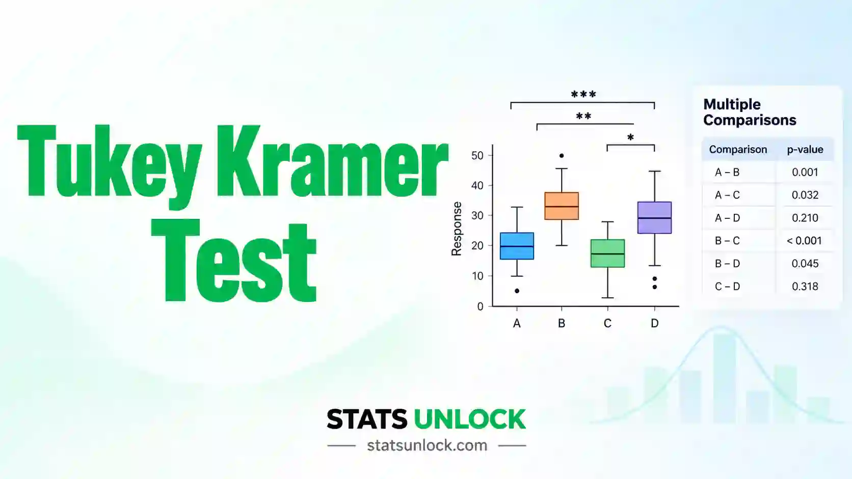

Tukey Kramer Test Calculator
Paste comma-separated numbers for each group or upload a CSV. This free Tukey Kramer test calculator finds which group means differ after a one-way ANOVA, even when the sample sizes are unequal, and gives adjusted p-values, confidence intervals, effect sizes and four charts.
⚡ 0. Quick Answer
The Tukey Kramer test is a post hoc test that compares every pair of group means after a one-way ANOVA when the groups have unequal sample sizes, while holding the overall chance of a false positive at 5%.
For each pair it divides the difference in means by a standard error built from the ANOVA error variance and both group sizes. The result, q, is compared with the studentized range distribution. With equal group sizes it gives exactly the same answer as the Tukey HSD test.
Rule of thumb: a pair differs when q is larger than the critical value q(α, k, N − k), or when the adjusted p-value is below 0.05. With 4 groups and 22 error degrees of freedom the critical value is 3.927.
Key takeaways
- The Tukey Kramer test is the version of Tukey HSD for unequal sample sizes, and it is what R, SciPy, SPSS and JMP run by default.
- With k groups there are k(k − 1) ÷ 2 comparisons, so 4 groups give 6 pairs and 6 groups give 15.
- It keeps the family-wise error rate at or below α = 0.05. Six uncorrected t-tests would push it to about 26%.
- It assumes normal residuals and equal variances. If the largest variance is more than 4 times the smallest, use Games-Howell instead.
- Report the mean difference, the 95% simultaneous confidence interval and the adjusted p-value for every pair, not only the significant ones.
📚 1. What Is the Tukey Kramer Test?
The Tukey Kramer test is a multiple comparison procedure. A one-way ANOVA tells you that at least one group mean differs from the others. It does not tell you which one. The Tukey Kramer post hoc test answers that second question by testing every possible pair of groups in one step.
John Tukey designed the original method in 1949 for groups of equal size. Clyde Kramer extended it in 1956 so that it also works when groups have different numbers of observations. That extension is the only difference between the two names. Many programs still print "Tukey HSD" on output that is really the Tukey Kramer HSD test.
What it measures. For each pair it measures how many standard errors apart the two means are. That number is called q, the studentized range statistic. A large q means the gap between two means is big compared with the noise inside the groups.
A worked one-liner. Fertilizer B plants averaged 69.86 cm from 7 plots and Control plants averaged 53.00 cm from 8 plots. The ANOVA error variance was 14.198. So SE = √[(14.198 ÷ 2) × (1 ÷ 7 + 1 ÷ 8)] = 1.379, and q = 16.857 ÷ 1.379 = 12.22. The critical value is 3.927, so the two groups clearly differ.
Who uses it. Agronomists comparing treatments in field trials, clinical researchers comparing dose groups, ecologists comparing habitats, teachers comparing class sections, and engineers comparing suppliers. In all of these the groups rarely end up the same size, which is exactly when to use the Tukey Kramer test.
Tukey HSD vs Tukey Kramer vs the alternatives
| Test | Group sizes | Variances | Compares | Use it when |
|---|---|---|---|---|
| Tukey HSD | Equal | Equal | All pairs | A balanced design with every pair of interest |
| Tukey Kramer | Equal or unequal | Equal | All pairs | Group sizes differ. This is the general case |
| Games-Howell | Equal or unequal | Unequal | All pairs | Levene's test fails or variances differ by more than 4 times |
| Dunnett | Equal or unequal | Equal | Each group vs one control | You only care about comparisons with a control |
| Bonferroni | Any | Depends on the test | A few chosen pairs | You planned a small number of comparisons in advance |
| Dunn test | Any | Not required | All pairs, on ranks | Data are not normal and you ran Kruskal-Wallis |
🧮 2. Set Up Your Data
Type one value per cell. Each column becomes a group, and the top row holds the group names. Empty cells are ignored, so columns can have different lengths.
📊 3. Results
🧠 4. Interpretation of Results, In Detail
4.1 What the Tukey Kramer test actually tells you
The test gives one answer per pair of groups: is the gap between these two means larger than chance alone would produce, once you allow for the fact that you looked at every pair? That last part matters. If you compare enough pairs, some gap will look big by luck. The Tukey Kramer test raises the bar so that the chance of even one false alarm across the whole set stays at your chosen level, usually 5%.
So a significant pair is a strong statement. It says this difference stood out even after the test was made stricter for all the looking you did. In the worked example, Fertilizer B beat the Control by 16.86 cm with an adjusted p below .001. You can say with confidence that B plants are taller.
4.2 How to read the mean difference and its sign
Each row shows the second group minus the first. A positive number means the second group has the higher mean. A negative number means it has the lower mean. The sign carries no judgement. It only tells you the direction. "Fertilizer C − Fertilizer B = −11.86" means C plants were 11.86 cm shorter than B plants on average.
Always read the difference in the units you measured. A difference of 11.86 cm on plants about 60 cm tall is large. The same number on trees 20 metres tall would not matter. The p-value cannot make that judgement for you.
4.3 The q statistic and the critical value
The q statistic is the difference in means divided by its standard error. It is a signal-to-noise ratio. A q of 5.91 means the two means are 5.91 standard errors apart. The critical value is the size of q you would need to call a pair different. It depends on three things: your alpha, the number of groups k, and the error degrees of freedom N − k.
More groups push the critical value up, because more pairs give chance more opportunities. With 22 error degrees of freedom the critical q is 2.93 for 2 groups, 3.55 for 3 groups, 3.93 for 4 groups and 4.20 for 5 groups. This is why adding groups you do not care about costs you power on the pairs you do care about.
4.4 Adjusted p-values and why they are larger than t-test p-values
The adjusted p-value answers this question: if all group means were truly equal, how often would the largest gap among all pairs be at least this big? Because it refers to the largest gap in the whole family, it is always bigger than the p-value from a plain t-test on the same two groups.
In the worked example, Fertilizer C against Control gives q = 3.29 and an adjusted p of .122. A simple two-sample t-test on those same two groups gives p = .066. Neither is below .05 here, but the gap between them shows the price of looking at six pairs. Never mix the two kinds of p-value in one table.
4.5 Simultaneous confidence intervals are the most useful output
Each interval gives a range of plausible values for the true difference. If the interval does not include zero, the pair is significant. The intervals are called simultaneous because all of them hold together with 95% confidence. That is a stronger promise than six separate 95% intervals, so each one is wider.
Read both ends. Fertilizer A against Control gives 8.50 cm with an interval from 2.85 to 14.15. The fertilizer helps, but the true gain might be as small as 3 cm or as large as 14 cm. If a 3 cm gain would not pay for the fertilizer, the significant result is not yet a decision.
4.6 What "not significant" does and does not mean
A pair that is not significant has not been shown to be equal. The test only says the data cannot separate the two groups. Fertilizer C against Fertilizer A gives a difference of −3.50 cm with an interval from −9.84 to 2.84. The true difference could be zero. It could also be nearly 10 cm. With only 5 and 6 plots, the study cannot tell.
Wide intervals around zero mean "we do not know". Narrow intervals around zero mean "any difference is small". Only the second one supports a claim that two groups are about the same.
4.7 Reading the compact letter display
Letters summarise the whole table in one line. Groups that share a letter are not significantly different. Groups with no letter in common are. In the example the letters are: Fertilizer B a, Fertilizer A b, Fertilizer C bc, Control c.
Fertilizer B stands alone at the top. Fertilizer C has two letters, b and c. It overlaps with Fertilizer A above it and with the Control below it, so it cannot be separated from either. Yet A and the Control do differ from each other. This pattern looks odd at first, but it is normal. It simply reflects that C sits in the middle with a small sample.
4.8 Effect sizes: how big, not only how sure
Eta squared is the share of all variation explained by the groups. In the example it is 0.779, so the fertilizer type accounts for about 78% of the variation in height. Omega squared, 0.741, is a slightly smaller and less biased version, and it is the better one to report for small samples.
Hedges g describes one pair. It is the mean difference divided by the pooled standard deviation, with a small-sample correction. By convention 0.2 is small, 0.5 is medium and 0.8 is large. Field experiments with tight control often give values far above 0.8, as this one does. That is fine. It means the groups barely overlap.
4.9 When the ANOVA and the Tukey Kramer test disagree
Sometimes the ANOVA is significant but no pair is. Sometimes a pair is significant but the ANOVA is not. Both can happen, because the two tests ask different questions. The F test looks at all means together. The Tukey Kramer test looks at the largest gap. Disagreement happens near the boundary, when p-values sit close to 0.05.
You do not need a significant ANOVA before running the Tukey Kramer test. The test controls the error rate on its own. Requiring both makes the procedure more conservative than it claims to be. If they disagree, report both honestly and treat the result as borderline.
4.10 Decision guide and common mistakes this calculator prevents
| What you see | What to conclude | What to do next |
|---|---|---|
| Adjusted p below alpha, interval far from zero | A clear difference | Report the difference, interval and effect size |
| Adjusted p below alpha, interval nearly touching zero | A real but possibly small difference | Report it, and discuss whether the lower limit matters in practice |
| Adjusted p between alpha and about 0.10 | Borderline | Do not claim a difference. Say the evidence is weak and more data are needed |
| Adjusted p well above alpha, wide interval | Inconclusive | Do not claim the groups are equal. Report the interval |
| Levene's test fails | The pooled variance is not valid | Switch to Games-Howell |
| Residuals not normal and groups small | p-values may be wrong | Transform the data or use Kruskal-Wallis with Dunn tests |
✍ 5. How to Write Your Results in Research
When reporting Tukey Kramer test results, readers need five things: the ANOVA result, the name of the post hoc test, why you chose it, the size and direction of each difference with its confidence interval, and the adjusted p-value. The five templates below fill themselves with your numbers after you run the analysis.
📌 Key conventions for this style
- Italicise F, p, M, SD, n and q in your word processor.
- Write p-values without a leading zero, and write p < .001 for anything smaller.
- Give the confidence interval in square brackets after the mean difference.
- Name the test as "Tukey-Kramer" when group sizes are unequal, not "Tukey HSD".
- Report non-significant pairs too, at least as a range of p-values.
📌 Key conventions for this style
- Justify the choice of post hoc test. Examiners ask why not Bonferroni or Games-Howell.
- Report both assumption checks with their test statistics.
- Give the MSE, the error degrees of freedom and the critical q so the analysis can be reproduced.
- Put the full pairwise table in the text or an appendix.
- Name the software and version used.
📌 Key conventions for this style
- No symbols, no test names, no p-values.
- Say "a real difference" or "we could not tell them apart", never "significant".
- Give the size of the gap in everyday units.
- Do not say groups are "the same" when the test was only inconclusive.
📌 Key conventions for this style
- Keep to the Objective, Methods, Results, Conclusion headings.
- State the family-wise alpha once in Methods.
- On a poster, show chart 1 with the letters and put this text beside it.
- Give the largest effect with its interval. Leave the full table for a handout.
📌 Key conventions for this style
- State the comparisons, the alpha and the decision rule before collecting data.
- Give every number needed to recompute the result: group sizes, MSE, degrees of freedom, critical q.
- List all pairs, not a selection.
- Say plainly if any comparison was added after seeing the data.
5.1 Methods section wording
Say what was compared, which test was used and why. A good sentence is: "Group means were compared with a one-way ANOVA followed by Tukey-Kramer post hoc tests, because all pairwise comparisons were of interest and group sizes were unequal. The family-wise error rate was set at .05."
5.2 Results sentence
Lead with the ANOVA, then the pairs. Give direction in words: "Fertilizer B produced taller plants than the Control". Follow with the numbers in brackets. Do not write "there was a significant difference between B and Control" without saying which was higher.
5.3 Table and figure conventions
A results table needs one row per pair with the mean difference, standard error, q or t, adjusted p and the confidence interval. A figure should show group means with intervals and the compact letters above each bar, as chart 1 does. State in the caption that groups sharing a letter do not differ by the Tukey-Kramer test at your alpha.
5.4 Discussion sentence
Link the size of the difference to its practical meaning. "The 16.9 cm gain from Fertilizer B is about a third of the control height, which is large enough to matter commercially." Mention any pairs that were inconclusive and what sample size would resolve them.
5.5 Reporting checklist
- ANOVA: F, both degrees of freedom, p and an effect size.
- The name "Tukey-Kramer" and the reason for using it.
- The family-wise alpha.
- For each pair: difference, confidence interval, adjusted p.
- Group n, mean and SD.
- Results of the normality and equal-variance checks.
- The software used.
∑ 6. Formulas Used
The Tukey Kramer test formula is built in seven steps. Each card below defines one quantity before the next card uses it.
🔀 7. Tukey Kramer Test Calculation Flowchart, Step by Step
This flowchart shows how the Tukey Kramer test is calculated step by step, from raw group data to a decision for each pair. Every box uses the worked example from this page: plant height in cm from a fertilizer trial with a Control and three fertilizers.
Check any box yourself: the Excel sheet in Section 9, the R script in Section 10 and the Python script in Section 11 all return MSE = 14.198, critical q = 3.927 and q = 12.22 for Fertilizer B against the Control.
📝 8. How to Use This Calculator
- Enter your data. Each group has its own box. Type or paste numbers separated by commas, exactly as the placeholder shows: 52, 48, 55, 61, 47, ... New lines, tabs, semicolons and spaces also work, so a column pasted from Excel is fine.
- Name each group. The name field above every box is editable. Type something meaningful such as Fertilizer A. The name appears in every table, all four charts and the exported report.
- Add or remove groups. Press Add group for more groups, up to 12. Each box has its own Clear and Remove button.
- Or upload a file. On the Upload tab choose a CSV or Excel file, then click the column names you want. Every column you click is loaded as a separate group. Files in long format, with one column of group names and one of values, are also supported.
- Try a sample dataset. Ten built-in datasets cover the cases that matter: a textbook example, a clear dose response, a borderline result, a null result, a small pilot, a large survey with a trivial effect and one where the assumptions fail.
- Describe the study. The study name, what was measured and the units are optional. They are used to write full sentences in the reports.
- Choose alpha. Leave it at 0.05 unless your field or your pre-registration says otherwise.
- Press Run Tukey-Kramer Test. Nothing is calculated until you do. Changing any input clears the results, so you never read numbers from old data.
- Read the assumption checks before the p-values. If Levene's test fails, the tool tells you to use Games-Howell. If it passes, read the pairwise table and chart 3.
- Copy the write-up and export. Section 5 fills five reporting styles with your numbers. The buttons under the charts save a text report or a print-ready PDF.
📈 9. How to Run the Tukey Kramer Test in Excel
Excel has no built-in function for the Tukey Kramer test, and the Analysis ToolPak does not offer it either. What Excel does well is the arithmetic: the group means, the pooled error variance, the standard error for each pair and the q statistic. The one thing Excel cannot do is look up the studentized range distribution. So you compute q in the sheet and compare it with a critical value from the table in Section 12, or from this calculator.
=ABS(C12-A12)/SQRT($H$4/2*(1/C11+1/A11)). If the answer is larger than the critical q, the pair differs.9.1 The functions you need
| You want | Excel function | Note |
|---|---|---|
| Group size | =COUNT(A2:A9) | Counts numbers only, so blank cells in a short column are ignored |
| Group mean | =AVERAGE(A2:A9) | Ignores blanks and text |
| Group variance | =VAR.S(A2:A9) | The sample version, dividing by n − 1. Never VAR.P here |
| Error degrees of freedom | =SUM(A11:D11)-COUNT(A11:D11) | N − k |
| MSE | =SUMPRODUCT(A11:D11-1,A13:D13)/H3 | Each variance weighted by its n − 1 |
| Standard error for a pair | =SQRT($H$4/2*(1/C11+1/A11)) | The Kramer form, valid for unequal n |
| q statistic | =ABS(K3)/L3 | Mean difference divided by the standard error |
| Whole ANOVA table | Data → Data Analysis → Anova: Single Factor | Analysis ToolPak. Enable it first under File → Options → Add-ins. "MS Within Groups" is the MSE |
| Critical q | No function exists | Use Table 12.1, or the free Real Statistics add-in function QCRIT |
=T.TEST(A2:A9,C2:C8,2,2) on every pair. Those p-values are not adjusted for multiple comparisons, and each one uses only two groups to estimate the variance. With 6 pairs the chance of at least one false positive rises from 5% to about 26%. That is the exact problem the Tukey Kramer test in Excel is meant to solve.9.2 Step by step
1 Put each group in its own column
Give every group one column with its name in row 1. Columns can have different lengths. Leave the unused cells empty, and never type 0 to fill a gap.
The fertilizer trial: Control has 8 values, Fertilizer A has 6, Fertilizer B has 7 and Fertilizer C has 5. Rows 1 to 9 hold all the data.
2 Summarise each group
Under the data, compute the size, mean and variance of every column. Type each formula once in column A and drag it across to column D.
=COUNT(A2:A9)=AVERAGE(A2:A9)=VAR.S(A2:A9)
Row 11 gives n = 8, 6, 7, 5. Row 12 gives the means 53.000, 61.500, 69.857, 58.000. Row 13 gives the variances 23.429, 11.500, 8.476, 10.000.
3 Compute the MSE
The MSE is the average of the group variances, weighted by each group's degrees of freedom. Build it in four cells so you can see every part.
H1: =COUNT(A11:D11)H2: =SUM(A11:D11)H3: =H2-H1H4: =SUMPRODUCT(A11:D11-1,A13:D13)/H3
k = 4, N = 26, error df = 22 and MSE = 14.198. The ToolPak ANOVA table shows the same number as "MS Within Groups". Type the critical value 3.927 into H5 from Table 12.1.
4 Build the pairwise table
Make one row per pair. For Fertilizer B against the Control, the difference, standard error and q are:
K3: =C12-A12L3: =SQRT($H$4/2*(1/C11+1/A11))M3: =ABS(K3)/L3
Fertilizer B minus Control: difference 16.857, standard error 1.379, q = 12.225. The dollar signs lock the MSE cell so the formula can be copied to the other rows. Change the two column letters for each new pair.
5 Add the confidence interval and the decision
The interval is the difference plus and minus the critical q times the standard error. The pair is significant when q is larger than the critical value.
N3: =K3-$H$5*L3O3: =K3+$H$5*L3P3: =IF(M3>$H$5,"Yes","No")
Four pairs say Yes and two say No, matching this calculator. The interval for Fertilizer B minus Control is 11.442 to 22.272.
9.3 The awkward cases
Adjusted p-values. Excel cannot compute the Tukey Kramer p-value, because it has no studentized range function. The closest built-in route is a Bonferroni p-value, which is a little larger and so a little more cautious:
=MIN(1, 6*T.DIST.2T(M3/SQRT(2), $H$3))
The 6 is the number of pairs, and dividing q by √2 turns it into a t statistic. For Fertilizer A against the Control this gives 0.0023, where the Tukey Kramer value is 0.0021. For Fertilizer C against the Control it gives 0.1772, against 0.1222. The classic mistake is to leave out the multiplication by the number of pairs.
A critical value for degrees of freedom not in the table. Printed tables skip values. For 22 degrees of freedom, take the entries for 20 (3.958) and 24 (3.901) and interpolate, or read the exact value 3.927 from this calculator.
Many groups. With 6 groups there are 15 pairs and 15 rows to type. Lay the means out in both a row and a column and fill a square table instead. Use INDEX to pick each mean and each n so one formula fills the whole grid.
The fastest check is to paste the same columns into the calculator on this page and compare the q values. They should agree to three decimal places.
9.4 Why your Excel answer might differ from R or Python
| Situation | What happens | Fix |
|---|---|---|
| You typed 0 in the empty cells of a short column | The zeros are counted as data, so n, the mean and the variance are all wrong | Delete them. Leave unused cells truly blank |
| Numbers stored as text | COUNT and AVERAGE skip them silently, so n is too small | Look for green triangles, then choose Convert to Number |
Used VAR.P or STDEV.P | The MSE comes out too small and q too large | Use VAR.S. R and SciPy both use n − 1 |
| Used √(MSE ÷ n) with one n for all pairs | That is the equal-n Tukey HSD formula. It is wrong for unequal groups | Use the Kramer standard error with both group sizes |
| Forgot to divide the MSE by 2 | You have computed t, not q. It is smaller by a factor of √2 | Either divide MSE by 2, or compare with qcrit ÷ √2 |
p-values from T.TEST are smaller than R's | They are unadjusted, and they use only two groups for the variance | Use the q comparison, or the Bonferroni formula in 9.3 |
| Critical q from a table for the wrong df | The decision can flip for pairs near the boundary | Interpolate, or take the exact value from this page |
| Rounding shown versus rounding stored | Typing a rounded MSE of 14.2 changes q in the third decimal | Always refer to the cell, never retype the number |
| Tool | How to run the Tukey Kramer test | Handles unequal n automatically? |
|---|---|---|
| Excel | By formula, as in 9.2 | Only if you use the Kramer standard error |
| Google Sheets | The same formulas work unchanged | Only if you use the Kramer standard error |
| R | TukeyHSD(aov(value ~ group)) | Yes |
| Python | scipy.stats.tukey_hsd(a, b, c, d) | Yes |
| SPSS | Analyze → Compare Means → One-Way ANOVA → Post Hoc → Tukey. SPSS applies the Kramer form when n is unequal | |
| JMP | Fit Y by X → Compare Means → All Pairs, Tukey HSD. JMP labels it Tukey-Kramer HSD | |
| Minitab | Stat → ANOVA → One-Way → Comparisons → Tukey | |
9.5 Charting the result in Excel
- Select the group names in row 1 and the means in row 12.
- Choose Insert → Charts → Clustered Column.
- Click the chart, press the + button, tick Error Bars, then choose More Options → Custom → Specify Value. Point it at a row holding
=T.INV.2T(0.05,$H$3)*SQRT($H$4/A11)for each group, which is the 95% margin. - Add a text box above each bar with its letter from the compact letter display, and say in the caption that groups sharing a letter do not differ.
- Remove the gridlines and the chart border, and label the y axis with the units.
Chart 1 in Section 3 of this page draws the same figure with the letters already placed, which is usually quicker than building it in Excel.
9.6 Excel errors you will probably hit
| Excel shows | Why | Fix |
|---|---|---|
#DIV/0! | A group has no numbers, or only one, so its variance cannot be computed | Every group needs at least 2 values. Check the ranges |
#VALUE! | A cell contains text such as "52 cm" or a stray space | Keep units in the header, not in the cells |
#NUM! | SQRT was given a negative number, usually from a wrong cell reference | Check that the MSE reference points at H4 and is locked with dollar signs |
#N/A | A lookup into the critical value table found no matching df | Interpolate between the two nearest rows |
#NAME? | You typed QCRIT or TUKEY without the add-in installed | Install the add-in, or type the critical value by hand |
| "Data Analysis" is missing from the Data tab | The Analysis ToolPak is not enabled | File → Options → Add-ins → Manage Excel Add-ins → tick Analysis ToolPak |
| q is the same for every pair | The group size references did not change when you copied the formula | Edit the two column letters in each row |
📈 10. How to Run the Tukey Kramer Test in R
The Tukey Kramer test in R is one line: TukeyHSD(aov(value ~ group, data = df)). The function is named for Tukey HSD, but it uses the Kramer standard error whenever group sizes differ, so there is nothing extra to switch on. The one-liner prints a table and stops there. The script below also checks the assumptions, shows the calculation by hand so every number can be traced, prints a plain-English verdict and saves one 300 dpi figure.
Rscript. Change only the groups <- list(...) block to use your own data. It uses base R only, so there is nothing to install.10.1 The complete script
R, base only, saves tukey_kramer_plot.png
# ============================================================
# Tukey-Kramer test with one publication-ready figure
# StatsUnlock - https://statsunlock.com/tukey-kramer-test-calculator/
# Base R only. No packages to install.
# ============================================================

# ---- 1. Your data ------------------------------------------
# Replace this list with your own groups, or read a long-format CSV:
#   df <- read.csv("data.csv")[, c("value", "group")]
#   df <- df[complete.cases(df), ]
groups <- list(
  "Control"      = c(52, 48, 55, 61, 47, 50, 58, 53),
  "Fertilizer A" = c(60, 57, 66, 63, 59, 64),
  "Fertilizer B" = c(68, 72, 65, 70, 74, 69, 71),
  "Fertilizer C" = c(56, 62, 58, 54, 60)
)
alpha <- 0.05
units <- "cm"

df <- stack(groups)
names(df) <- c("value", "group")
df$group <- factor(df$group, levels = names(groups))   # keep your order, not alphabetical

# ---- 2. One-way ANOVA and the pooled error variance --------
fit      <- aov(value ~ group, data = df)
tab      <- summary(fit)[[1]]
k        <- nlevels(df$group)
N        <- nrow(df)
df_error <- tab[["Df"]][2]
mse      <- tab[["Mean Sq"]][2]
F_val    <- tab[["F value"]][1]
p_anova  <- tab[["Pr(>F)"]][1]
eta2     <- tab[["Sum Sq"]][1] / sum(tab[["Sum Sq"]])

# ---- 3. The built-in Tukey-Kramer test ---------------------
tk     <- TukeyHSD(fit, conf.level = 1 - alpha)$group
q_crit <- qtukey(1 - alpha, nmeans = k, df = df_error)

# ---- 4. The same thing by hand, so every number is visible -
n  <- tapply(df$value, df$group, length)
m  <- tapply(df$value, df$group, mean)
pr <- combn(levels(df$group), 2)
hand <- t(apply(pr, 2, function(p) {
  d  <- unname(m[p[2]] - m[p[1]])
  se <- unname(sqrt(mse / 2 * (1 / n[p[1]] + 1 / n[p[2]])))   # the Kramer standard error
  q  <- abs(d) / se
  c(diff = d, se = se, q = q, p = ptukey(q, k, df_error, lower.tail = FALSE))
}))
rownames(hand) <- paste(pr[2, ], pr[1, ], sep = " - ")
stopifnot(all(abs(hand[, "p"] - tk[, "p adj"]) < 1e-6))

# ---- 5. Assumption checks ----------------------------------
sw  <- shapiro.test(residuals(fit))
z   <- abs(df$value - ave(df$value, df$group, FUN = median))
lev <- anova(lm(z ~ df$group))          # Levene test, median centred

# ---- 6. Printed summary ------------------------------------
cat(sprintf("k = %d, N = %d, n per group = %s\n", k, N, paste(n, collapse = ", ")))
cat(sprintf("ANOVA: F(%d, %d) = %.4f, p = %.3g, eta squared = %.4f\n",
            k - 1, df_error, F_val, p_anova, eta2))
cat(sprintf("MSE = %.4f, critical q(%d, %d) = %.4f\n\n", mse, k, df_error, q_crit))
out <- cbind(hand[, c("diff", "se", "q")], "p adj" = tk[, "p adj"],
             lwr = tk[, "lwr"], upr = tk[, "upr"])
print(round(out, 4))
cat(sprintf("\nShapiro-Wilk on residuals: W = %.4f, p = %.4f\n", sw$statistic, sw$p.value))
cat(sprintf("Levene (median): F = %.4f, p = %.4f\n", lev[["F value"]][1], lev[["Pr(>F)"]][1]))
n_sig <- sum(tk[, "p adj"] < alpha)
ok    <- sw$p.value >= 0.05 && lev[["Pr(>F)"]][1] >= 0.05
cat(sprintf("\nVerdict: %d of %d pairs differ at family-wise alpha = %.2f. %s\n",
            n_sig, nrow(tk), alpha,
            if (ok) "Assumptions hold, so report these results."
            else "An assumption failed, so confirm with Games-Howell."))

# ---- 7. One figure: simultaneous confidence intervals ------
png("tukey_kramer_plot.png", width = 2700,
    height = round(300 * (0.62 * nrow(tk) + 2.6)), res = 300)
par(mar = c(5, 13, 5, 2), family = "sans")
ypos <- rev(seq_len(nrow(tk)))
sig  <- tk[, "p adj"] < alpha
plot(NA, xlim = range(c(tk[, "lwr"], tk[, "upr"], 0)),
     ylim = c(0.5, nrow(tk) + 0.5), yaxt = "n", bty = "n", ylab = "",
     xlab = sprintf("Difference in means (%s) with %.0f%% simultaneous CI",
                    units, 100 * (1 - alpha)))
grid(nx = NULL, ny = NA, col = "#e5e7eb", lty = 1)
abline(v = 0, lty = 2, lwd = 1.6, col = "#111827")
segments(tk[, "lwr"], ypos, tk[, "upr"], ypos, lwd = 7, lend = 1,
         col = ifelse(sig, "#7e22ce", "#94a3b8"))
points(tk[, "diff"], ypos, pch = 21, bg = "#111827", col = "white", cex = 1.5)
axis(2, at = ypos, labels = rownames(hand), las = 1, tick = FALSE, cex.axis = 0.85)
title(main = "Tukey-Kramer test: pairwise differences", adj = 0, line = 2.6, cex.main = 1.15)
title(main = sprintf("F(%d, %d) = %.2f, MSE = %.2f, critical q = %.3f",
                     k - 1, df_error, F_val, mse, q_crit),
      adj = 0, line = 1.2, cex.main = 0.95, font.main = 1)
dev.off()
cat("\nSaved tukey_kramer_plot.png\n")
Run it with Rscript tukey_kramer.R from a terminal, or paste it into the RStudio console. The figure is saved as tukey_kramer_plot.png in your working directory, which you can find with getwd(). The script contains no random numbers, so there is nothing to seed and the figure is identical on every run.
10.2 What each part does
| Line or function | What it does, and why it is there |
|---|---|
| groups <- list(...) | Holds one numeric vector per group. A list is used because the groups have different lengths, which a data frame of columns cannot hold. |
| stack(groups) | Turns the list into long format: one row per observation, with a value column and a group factor. aov() needs this shape. The formula value ~ group does not work on separate vectors. |
| read.csv() and complete.cases() | The commented alternative for a real file. Dropping rows with NA first matters, because aov() removes them silently and your n changes without warning. |
| factor(df$group, levels = ...) | Fixes the group order. Without it R sorts groups alphabetically, which changes the order and the sign of every difference. |
| aov(value ~ group) | Fits the one-way ANOVA. The Mean Sq of the residual row is the MSE that every comparison uses. |
| TukeyHSD(fit) | Runs all pairwise comparisons. Despite the name it applies the Tukey-Kramer adjustment for unequal n. Each row is the later group minus the earlier one. |
| qtukey(1 - alpha, k, df) | The critical value of the studentized range. This is the number Excel cannot compute. |
| ptukey(q, k, df, lower.tail = FALSE) | The adjusted p-value for one q. lower.tail = FALSE gives the upper tail directly, which is more accurate than 1 - ptukey() for tiny p-values. |
| combn(levels, 2) | Lists every pair of groups once, in the same order that TukeyHSD uses, so the by-hand table lines up with the built-in one. |
| stopifnot(...) | Stops the script if the by-hand p-values and the built-in ones disagree. It is a safety check that the formula in Section 6 is what R really computes. |
| shapiro.test(residuals(fit)) | Tests normality on the residuals, not the raw data. Raw data from groups with different means will look non-normal even when each group is perfectly normal. |
| ave(..., FUN = median) | Gives each observation its own group median. The absolute deviations from it feed the median-centred Levene test, which base R does not have as a function. |
| png(..., res = 300) | Opens a file device at print quality. Without res = 300 you get a blurry 72 dpi image. |
| segments() and points() | Draw each confidence interval as a thick line and each difference as a dot. Purple means significant, grey means not. |
| dev.off() | Closes the device and writes the file. Forgetting this leaves an empty or locked PNG. |
10.3 What the figure shows
The figure has one horizontal line per pair. The dot is the difference in means and the line is its 95% simultaneous confidence interval. The dashed vertical line marks zero. Any interval that does not touch the dashed line is a significant difference, and it is drawn in purple.
For the fertilizer trial, four intervals sit clear of zero and two cross it. The widest intervals belong to pairs that include Fertilizer C, the group with only 5 plots. That is the Kramer standard error at work: smaller groups get wider intervals.
10.4 Common R problems and fixes
| Symptom | Cause | Fix |
|---|---|---|
TukeyHSD says "no factors in the fitted model" | The group column is numeric, for example doses 10, 20, 40 | Wrap it: aov(value ~ factor(group)) |
| Groups appear in alphabetical order | R sorts factor levels by default | Set the order with factor(x, levels = c(...)) |
| The signs of the differences are reversed compared with another program | R reports the later level minus the earlier one | Nothing is wrong. Reverse the factor levels if you want the other direction |
| N is smaller than expected | aov() dropped rows containing NA without telling you | Clean first with complete.cases() and check nrow() |
Error in aov() about object not found | Two separate vectors were passed instead of a long data frame | Use stack() as the script does |
| p-values differ from SPSS in the last digit | Different numerical integration of the studentized range | Ignore differences beyond the fourth decimal place |
| The plot labels are cut off on the left | The left margin is too narrow for long group names | Increase the second number in par(mar = c(5, 13, 5, 2)) |
| The PNG is empty | dev.off() was never called | Run while (dev.cur() > 1) dev.off() |
10.5 Useful one-liners
| You want | R code |
|---|---|
| The test in one line | TukeyHSD(aov(value ~ group, data = df)) |
| 99% intervals instead of 95% | TukeyHSD(fit, conf.level = 0.99) |
| The built-in interval plot | plot(TukeyHSD(fit), las = 1) |
| A critical value | qtukey(0.95, nmeans = 4, df = 22) |
| An adjusted p-value from q | ptukey(5.907, 4, 22, lower.tail = FALSE) |
| Compact letters, with the multcompView package | multcompView::multcompLetters4(fit, TukeyHSD(fit)) |
| Games-Howell for unequal variances, with rstatix | rstatix::games_howell_test(df, value ~ group) |
| Save the table as a CSV | write.csv(TukeyHSD(fit)$group, "tukey_kramer.csv") |
📈 11. How to Run the Tukey Kramer Test in Python
In Python the test is scipy.stats.tukey_hsd(a, b, c, d), available from SciPy 1.8. Like R, the function is named for Tukey HSD but applies the Kramer adjustment when the samples differ in size. The script below is complete and runnable. It computes every number by hand, confirms them against SciPy's own result, checks the assumptions, prints a verdict and saves one 300 dpi figure.
groups = {...} dictionary. The script was run with SciPy 1.18 to produce the numbers on this page.Install with pip install numpy scipy matplotlib. You need SciPy 1.8 or newer. Check with python -c "import scipy; print(scipy.__version__)".
11.1 The complete script
Python 3, saves tukey_kramer_plot.png
# ============================================================
# Tukey-Kramer test with one publication-ready figure
# StatsUnlock - https://statsunlock.com/tukey-kramer-test-calculator/
# ============================================================

import numpy as np
import matplotlib.pyplot as plt
from itertools import combinations
from scipy import stats

# ---- 1. Your data ------------------------------------------
# Replace this dictionary with your own groups, or read a CSV:
#   import pandas as pd
#   df = pd.read_csv("data.csv").dropna(subset=["group", "value"])
#   groups = {g: d["value"].to_numpy(float) for g, d in df.groupby("group")}
groups = {
    "Control":      [52, 48, 55, 61, 47, 50, 58, 53],
    "Fertilizer A": [60, 57, 66, 63, 59, 64],
    "Fertilizer B": [68, 72, 65, 70, 74, 69, 71],
    "Fertilizer C": [56, 62, 58, 54, 60],
}
alpha = 0.05
units = "cm"

names = list(groups)
data  = [np.asarray(groups[g], dtype=float) for g in names]
k     = len(data)
n     = np.array([len(x) for x in data])
N     = n.sum()
means = np.array([x.mean() for x in data])

# ---- 2. One-way ANOVA and the pooled error variance --------
F, p_anova = stats.f_oneway(*data)
df_error   = N - k
mse        = sum(((x - x.mean()) ** 2).sum() for x in data) / df_error
ss_between = sum(len(x) * (x.mean() - np.concatenate(data).mean()) ** 2 for x in data)
eta2       = ss_between / (ss_between + mse * df_error)

# ---- 3. Tukey-Kramer by hand, so every number is visible ---
q_crit = stats.studentized_range.ppf(1 - alpha, k, df_error)
rows = []
for i, j in combinations(range(k), 2):
    diff = means[j] - means[i]
    se   = np.sqrt(mse / 2 * (1 / n[i] + 1 / n[j]))   # the Kramer standard error
    q    = abs(diff) / se
    p    = stats.studentized_range.sf(q, k, df_error)
    rows.append((names[j], names[i], diff, se, q, p, diff - q_crit * se, diff + q_crit * se))

# ---- 4. Cross-check against SciPy's built-in ----------------
res = stats.tukey_hsd(*data)        # uses the Kramer form when n is unequal
for b, a, diff, se, q, p, lo, hi in rows:
    i, j = names.index(a), names.index(b)
    assert abs(res.pvalue[j, i] - p) < 1e-6

# ---- 5. Assumption checks ----------------------------------
resid       = np.concatenate([x - x.mean() for x in data])
W, p_norm   = stats.shapiro(resid)
L, p_levene = stats.levene(*data, center="median")

# ---- 6. Printed summary ------------------------------------
print(f"k = {k}, N = {N}, n per group = {n.tolist()}")
print(f"ANOVA: F({k - 1}, {df_error}) = {F:.4f}, p = {p_anova:.3g}, eta squared = {eta2:.4f}")
print(f"MSE = {mse:.4f}, critical q({k}, {df_error}) = {q_crit:.4f}\n")
print(f"{'comparison':<30}{'diff':>9}{'SE':>9}{'q':>9}{'p adj':>9}{'CI low':>9}{'CI high':>9}")
for b, a, diff, se, q, p, lo, hi in rows:
    flag = "*" if p < alpha else ""
    print(f"{b + ' - ' + a:<30}{diff:>9.4f}{se:>9.4f}{q:>9.4f}{p:>9.4f}{lo:>9.4f}{hi:>9.4f} {flag}")
print(f"\nShapiro-Wilk on residuals: W = {W:.4f}, p = {p_norm:.4f}")
print(f"Levene (median): F = {L:.4f}, p = {p_levene:.4f}")
n_sig = sum(r[5] < alpha for r in rows)
ok = p_norm >= 0.05 and p_levene >= 0.05
print(f"\nVerdict: {n_sig} of {len(rows)} pairs differ at family-wise alpha = {alpha}.",
      "Assumptions hold, so report these results." if ok
      else "An assumption failed, so confirm with Games-Howell.")

# ---- 7. One figure: simultaneous confidence intervals ------
fig, ax = plt.subplots(figsize=(8.5, 0.62 * len(rows) + 2.2))
ypos = np.arange(len(rows))[::-1]
for y, (b, a, diff, se, q, p, lo, hi) in zip(ypos, rows):
    colour = "#7e22ce" if p < alpha else "#94a3b8"
    ax.plot([lo, hi], [y, y], color=colour, lw=6, solid_capstyle="round", alpha=0.75, zorder=2)
    ax.plot(diff, y, "o", color="#111827", ms=7, mec="white", mew=1.3, zorder=3)
ax.axvline(0, color="#111827", lw=1.4, ls="--", zorder=1)
ax.set_yticks(ypos)
ax.set_yticklabels([f"{b} - {a}" for b, a, *_ in rows], fontsize=10)
ax.set_xlabel(f"Difference in means ({units}) with {100 * (1 - alpha):.0f}% simultaneous CI", fontsize=11)
ax.set_title("Tukey-Kramer test: pairwise differences\n"
             f"F({k - 1}, {df_error}) = {F:.2f}, MSE = {mse:.2f}, critical q = {q_crit:.3f}",
             fontsize=12, fontweight="bold", loc="left")
ax.grid(axis="x", alpha=0.25, zorder=0)
ax.spines[["top", "right"]].set_visible(False)
fig.savefig("tukey_kramer_plot.png", dpi=300, bbox_inches="tight")
print("\nSaved tukey_kramer_plot.png")
Run it with python tukey_kramer.py. In Jupyter, add plt.show() after the savefig line to display the figure as well. The script contains no random numbers, so there is nothing to seed.
11.2 What each part does
| Line or function | What it does, and why it is there |
|---|---|
| groups = {...} | A dictionary of lists, one per group. Lists can be different lengths, which is the whole point of the Kramer version. |
| np.asarray(..., dtype=float) | Converts each list to a float array. Forcing floats avoids integer arithmetic surprises. |
| pd.read_csv(...).dropna(...) | The commented alternative for a real file in long format. Drop missing values first, because np.mean returns nan if even one value is nan. |
| stats.f_oneway(*data) | The one-way ANOVA. The star unpacks the list so each group is passed as its own argument. |
| mse | The pooled within-group variance: the squared deviations from each group's own mean, summed and divided by N − k. SciPy does not return it, so it is computed by hand. |
| studentized_range.ppf(1 - alpha, k, df) | The critical value. This is the function Excel lacks. |
| np.sqrt(mse / 2 * (1/n[i] + 1/n[j])) | The Kramer standard error. Both group sizes appear, so every pair has its own value. |
| studentized_range.sf(q, k, df) | The adjusted p-value. sf is the survival function, 1 minus the CDF, computed accurately in the tail. |
| stats.tukey_hsd(*data) | SciPy's built-in version. Its pvalue attribute is a k by k matrix. The assert confirms the by-hand numbers match it. |
| stats.shapiro(resid) | Normality test on the residuals, not on the pooled raw data. |
| stats.levene(*data, center="median") | The Brown-Forsythe form of Levene's test. center="median" is SciPy's default, written out so nobody changes it by accident. |
| f"{value:>9.4f}" | Formats a number right-aligned in 9 characters with 4 decimals, so the printed table lines up. |
| ax.plot([lo, hi], [y, y]) | Draws one confidence interval as a thick horizontal line. |
| savefig(dpi=300, bbox_inches="tight") | Writes the file at print resolution and trims the white border. |
11.3 What the figure shows
The same figure as the R script: one line per pair, with the difference as a dot and its 95% simultaneous confidence interval as a bar. Purple bars are significant, grey bars are not, and the dashed line marks zero.
Reading it takes a few seconds. Four bars sit entirely on one side of zero. Two bars cross it: Fertilizer C against the Control, and Fertilizer C against Fertilizer A. Both involve the smallest group, and both have the widest bars.
11.4 Common Python problems and fixes
| Symptom | Cause | Fix |
|---|---|---|
AttributeError: module 'scipy.stats' has no attribute 'tukey_hsd' | SciPy is older than 1.8 | pip install --upgrade scipy |
Every result is nan | A group contains a missing value | Remove it with x = x[~np.isnan(x)] before running |
| The signs are reversed compared with R | tukey_hsd prints group i minus group j for every ordered pair | Read the row for the direction you want. The script reports later minus earlier, like R |
| Standard deviation differs from Excel | NumPy defaults to ddof=0, the population formula | Use np.std(x, ddof=1) to match STDEV.S and R |
pairwise_tukeyhsd from statsmodels gives a slightly different p | Older statsmodels versions interpolate from a table | Prefer scipy.stats.tukey_hsd, which integrates the distribution directly |
TypeError from f_oneway | The list of groups was passed without the star | Write stats.f_oneway(*data) |
| Nothing appears when the script runs | A non-interactive backend, which is normal on servers | The figure is saved to file. Add plt.show() to display it |
| The y-axis labels are cut off | Long group names | bbox_inches="tight" already handles this in the saved file |
11.5 Useful one-liners
| You want | Python code |
|---|---|
| The test in one line | print(stats.tukey_hsd(a, b, c, d)) |
| The matrix of adjusted p-values | stats.tukey_hsd(a, b, c, d).pvalue |
| 99% simultaneous intervals | res.confidence_interval(confidence_level=0.99) |
| A critical value | stats.studentized_range.ppf(0.95, 4, 22) |
| An adjusted p-value from q | stats.studentized_range.sf(5.907, 4, 22) |
| From a long-format data frame | stats.tukey_hsd(*[g["value"] for _, g in df.groupby("group")]) |
| With statsmodels | pairwise_tukeyhsd(df["value"], df["group"]).summary() |
| Games-Howell for unequal variances, with pingouin | pingouin.pairwise_gameshowell(df, dv="value", between="group") |
TukeyHSD applies the same formula, so its table should match to four decimals. If your two results disagree, the cause is almost always missing values handled differently or groups in a different order.📋 12. Reference Tables
12.1 Critical values of the studentized range, α = 0.05
| Error df | k = 2 | k = 3 | k = 4 | k = 5 | k = 6 | k = 7 | k = 8 | k = 9 | k = 10 |
|---|---|---|---|---|---|---|---|---|---|
| 5 | 3.635 | 4.602 | 5.218 | 5.673 | 6.033 | 6.330 | 6.582 | 6.801 | 6.995 |
| 6 | 3.460 | 4.339 | 4.896 | 5.305 | 5.628 | 5.895 | 6.122 | 6.319 | 6.493 |
| 8 | 3.261 | 4.041 | 4.529 | 4.886 | 5.167 | 5.399 | 5.596 | 5.767 | 5.918 |
| 10 | 3.151 | 3.877 | 4.327 | 4.654 | 4.912 | 5.124 | 5.304 | 5.460 | 5.598 |
| 12 | 3.081 | 3.773 | 4.199 | 4.508 | 4.750 | 4.950 | 5.119 | 5.265 | 5.395 |
| 15 | 3.014 | 3.673 | 4.076 | 4.367 | 4.595 | 4.782 | 4.940 | 5.077 | 5.198 |
| 20 | 2.950 | 3.578 | 3.958 | 4.232 | 4.445 | 4.620 | 4.768 | 4.895 | 5.008 |
| 22 | 2.933 | 3.553 | 3.927 | 4.196 | 4.405 | 4.577 | 4.722 | 4.847 | 4.957 |
| 24 | 2.919 | 3.532 | 3.901 | 4.166 | 4.373 | 4.541 | 4.684 | 4.807 | 4.915 |
| 30 | 2.888 | 3.486 | 3.845 | 4.102 | 4.301 | 4.464 | 4.601 | 4.720 | 4.824 |
| 40 | 2.858 | 3.442 | 3.791 | 4.039 | 4.232 | 4.388 | 4.521 | 4.634 | 4.735 |
| 60 | 2.829 | 3.399 | 3.737 | 3.977 | 4.163 | 4.314 | 4.441 | 4.550 | 4.646 |
| 120 | 2.800 | 3.356 | 3.685 | 3.917 | 4.096 | 4.241 | 4.363 | 4.468 | 4.560 |
| ∞ | 2.772 | 3.314 | 3.633 | 3.858 | 4.030 | 4.170 | 4.286 | 4.387 | 4.474 |
Conclusion: find your number of groups across the top and your error degrees of freedom, N − k, down the side. A pair differs when its q is larger than the table value. Values were computed from the studentized range distribution with SciPy and agree with published tables.
12.2 Critical values of the studentized range, α = 0.01
| Error df | k = 2 | k = 3 | k = 4 | k = 5 | k = 6 | k = 7 | k = 8 | k = 9 | k = 10 |
|---|---|---|---|---|---|---|---|---|---|
| 5 | 5.702 | 6.976 | 7.804 | 8.421 | 8.913 | 9.321 | 9.669 | 9.971 | 10.239 |
| 6 | 5.243 | 6.331 | 7.033 | 7.556 | 7.972 | 8.318 | 8.612 | 8.869 | 9.097 |
| 8 | 4.745 | 5.635 | 6.204 | 6.625 | 6.959 | 7.237 | 7.474 | 7.680 | 7.863 |
| 10 | 4.482 | 5.270 | 5.769 | 6.136 | 6.428 | 6.669 | 6.875 | 7.054 | 7.213 |
| 12 | 4.320 | 5.046 | 5.502 | 5.836 | 6.101 | 6.320 | 6.507 | 6.670 | 6.814 |
| 15 | 4.167 | 4.836 | 5.252 | 5.556 | 5.796 | 5.994 | 6.162 | 6.309 | 6.438 |
| 20 | 4.024 | 4.639 | 5.018 | 5.293 | 5.510 | 5.688 | 5.839 | 5.970 | 6.086 |
| 22 | 3.986 | 4.588 | 4.957 | 5.225 | 5.435 | 5.608 | 5.754 | 5.882 | 5.994 |
| 24 | 3.955 | 4.546 | 4.907 | 5.168 | 5.373 | 5.542 | 5.685 | 5.809 | 5.919 |
| 30 | 3.889 | 4.455 | 4.799 | 5.048 | 5.242 | 5.401 | 5.536 | 5.653 | 5.756 |
| 40 | 3.825 | 4.367 | 4.695 | 4.931 | 5.114 | 5.265 | 5.392 | 5.502 | 5.599 |
| 60 | 3.762 | 4.282 | 4.594 | 4.818 | 4.991 | 5.133 | 5.253 | 5.356 | 5.447 |
| 120 | 3.702 | 4.200 | 4.497 | 4.709 | 4.872 | 5.005 | 5.118 | 5.214 | 5.299 |
| ∞ | 3.643 | 4.120 | 4.403 | 4.603 | 4.757 | 4.882 | 4.987 | 5.078 | 5.157 |
Conclusion: the stricter 1% level needs a q about 20% to 35% larger once there are 20 or more error degrees of freedom, and much larger with fewer. Use it when a false positive would be costly.
12.3 Why a correction is needed: error rate from uncorrected t-tests
| Groups k | Pairs k(k − 1) ÷ 2 | Chance of at least one false positive, uncorrected | With the Tukey Kramer test |
|---|---|---|---|
| 2 | 1 | 5.0% | 5.0% or less |
| 3 | 3 | 14.3% | 5.0% or less |
| 4 | 6 | 26.5% | 5.0% or less |
| 5 | 10 | 40.1% | 5.0% or less |
| 6 | 15 | 53.7% | 5.0% or less |
| 8 | 28 | 76.2% | 5.0% or less |
| 10 | 45 | 90.1% | 5.0% or less |
Conclusion: with 5 groups, ten uncorrected t-tests give about a 40% chance of at least one false positive. The Tukey Kramer multiple comparison test holds that figure at 5% however many groups you have.
12.4 Effect size interpretation bands
| Effect size | Small | Medium | Large | Used for |
|---|---|---|---|---|
| Eta squared η² | 0.01 | 0.06 | 0.14 | The whole ANOVA: share of variance explained |
| Omega squared ω² | 0.01 | 0.06 | 0.14 | The same, with less bias in small samples |
| Cohen's f | 0.10 | 0.25 | 0.40 | Power analysis for ANOVA |
| Hedges g or Cohen's d | 0.20 | 0.50 | 0.80 | One pair of groups |
Conclusion: these are Cohen's general conventions. Many fields see larger effects as routine, especially controlled laboratory and field experiments, so compare with published values in your own area where you can.
12.5 Which post hoc test should you use?
| Your situation | Use | Why |
|---|---|---|
| All pairs, equal variances, equal n | Tukey HSD | Exact control of the family-wise error rate |
| All pairs, equal variances, unequal n | Tukey Kramer | Proven never to exceed alpha, and only slightly conservative |
| All pairs, unequal variances | Games-Howell | Uses a separate variance and Welch degrees of freedom for each pair |
| Each treatment against one control | Dunnett | Fewer comparisons, so more power for each one |
| A few comparisons planned in advance | Bonferroni or Holm | More powerful than Tukey Kramer when the list is short |
| Complex contrasts, such as two groups against three | Scheffé | Covers every possible contrast, at a cost in power |
| Data not normal, Kruskal-Wallis was used | Dunn test | Works on ranks and needs no normality |
| The same subjects measured in every condition | Paired comparisons with Holm | Tukey Kramer assumes independent groups |
Conclusion: choose the Tukey Kramer test when you want every pair, the variances are similar and the groups are independent. That covers most one-way designs.
12.6 Assumption check thresholds
| Check | Pass | Caution | Fail |
|---|---|---|---|
| Shapiro-Wilk p on residuals | p ≥ 0.05 | p < 0.05 with 15 or more per group | p < 0.05 with small groups |
| Levene p, median centred | p ≥ 0.05 | none | p < 0.05 |
| Largest variance ÷ smallest variance | up to 4 | 4 to 9 | above 9 |
| Smallest group size | 5 or more | 3 or 4 | 1 |
| Largest n ÷ smallest n | up to 2 | above 2 with unequal variances | none on its own |
Conclusion: unequal variances are the serious problem, and they are most damaging when the small groups are the ones with the large variances. Unequal group sizes alone are not a problem for this test.
12.7 Smallest detectable difference by group size
| n per group | k = 3 | k = 4 | k = 5 | k = 6 |
|---|---|---|---|---|
| 3 | 2.51 | 2.61 | 2.69 | 2.74 |
| 4 | 1.97 | 2.10 | 2.18 | 2.25 |
| 5 | 1.69 | 1.81 | 1.89 | 1.96 |
| 6 | 1.50 | 1.62 | 1.70 | 1.76 |
| 8 | 1.26 | 1.37 | 1.44 | 1.49 |
| 10 | 1.11 | 1.20 | 1.27 | 1.32 |
| 15 | 0.89 | 0.97 | 1.02 | 1.06 |
| 20 | 0.76 | 0.83 | 0.88 | 0.92 |
| 30 | 0.62 | 0.67 | 0.71 | 0.74 |
| 50 | 0.47 | 0.52 | 0.55 | 0.57 |
Conclusion: each entry is the smallest difference between two means that would be significant at α = 0.05, in units of the within-group standard deviation, for equal groups of size n. With 4 groups of 5, two means must be about 1.8 standard deviations apart. With 4 groups of 30 the figure drops to about 0.67. Small studies can only confirm large effects.
📈 13. Example Results
Eight worked examples of the Tukey Kramer test, each with real numbers you can reproduce by choosing the matching sample dataset in Section 2. Every Tukey Kramer test example shows what the result looks like and how to write it up.
Four fertilizers in a greenhouse trial
The worked example used in every section of this page.
Twenty-six plots received a Control or one of three fertilizers. Some plots were lost, so the groups ended with 8, 6, 7 and 5 plots. Sample dataset 1 in the calculator.
| Comparison | Mean diff | q | Adjusted p | 95% CI | Significant |
|---|---|---|---|---|---|
| Fertilizer A − Control | 8.50 | 5.907 | 0.0021 | 2.85 to 14.15 | Yes |
| Fertilizer B − Control | 16.86 | 12.225 | < 0.0001 | 11.44 to 22.27 | Yes |
| Fertilizer C − Control | 5.00 | 3.292 | 0.1222 | −0.96 to 10.96 | No |
| Fertilizer B − Fertilizer A | 8.36 | 5.638 | 0.0032 | 2.54 to 14.18 | Yes |
| Fertilizer C − Fertilizer A | −3.50 | 2.169 | 0.4352 | −9.84 to 2.84 | No |
| Fertilizer C − Fertilizer B | −11.86 | 7.600 | 0.0001 | −17.98 to −5.73 | Yes |
Assumption checks: Shapiro-Wilk W = 0.980, p = .868; Levene F(3, 22) = 0.87, p = .473; variance ratio 2.8.
What it means: Fertilizer B is clearly best and stands apart from every other group. Fertilizer A beats the Control. Fertilizer C sits in the middle and cannot be separated from A or from the Control, mainly because it has only 5 plots.
How to write it: A one-way ANOVA showed a significant effect of group on plant height, F(3, 22) = 25.83, p < .001, η² = .78. Tukey-Kramer post hoc tests showed that Fertilizer B was higher than Control (mean difference = 16.86 cm, 95% CI [11.44, 22.27], p < .001). In total 4 of 6 pairwise comparisons were significant.
A dose-response trial for blood pressure
Large, ordered differences with one adjacent pair left unresolved.
Forty-five patients received a placebo or one of three doses. The outcome is the drop in systolic blood pressure after eight weeks. Sample dataset 2 in the calculator.
| Comparison | Mean diff | q | Adjusted p | 95% CI | Significant |
|---|---|---|---|---|---|
| 10 mg − Placebo | 5.00 | 3.887 | 0.0423 | 0.13 to 9.87 | Yes |
| 20 mg − Placebo | 8.57 | 6.811 | 0.0001 | 3.80 to 13.33 | Yes |
| 40 mg − Placebo | 17.11 | 12.969 | < 0.0001 | 12.11 to 22.10 | Yes |
| 20 mg − 10 mg | 3.57 | 2.774 | 0.2192 | −1.30 to 8.44 | No |
| 40 mg − 10 mg | 12.11 | 8.995 | < 0.0001 | 7.01 to 17.21 | Yes |
| 40 mg − 20 mg | 8.54 | 6.475 | 0.0002 | 3.55 to 13.54 | Yes |
Assumption checks: Shapiro-Wilk W = 0.980, p = .609; Levene F(3, 41) = 0.32, p = .814; variance ratio 1.8.
What it means: The response rises with dose and five of six pairs differ. The one exception is 10 mg against 20 mg: the gap of 3.6 mmHg is real in the sample but too small to confirm with 11 and 12 patients.
How to write it: A one-way ANOVA showed a significant effect of group on reduction in systolic blood pressure, F(3, 41) = 29.48, p < .001, η² = .68. Tukey-Kramer post hoc tests showed that 40 mg was higher than Placebo (mean difference = 17.11 mmHg, 95% CI [12.11, 22.10], p < .001). In total 5 of 6 pairwise comparisons were significant.
Four teaching methods and exam scores
A significant ANOVA where only one pair survives adjustment.
Forty-seven students in four class sections of different sizes sat the same exam after different teaching formats. Sample dataset 3 in the calculator.
| Comparison | Mean diff | q | Adjusted p | 95% CI | Significant |
|---|---|---|---|---|---|
| Flipped − Lecture | 2.55 | 1.155 | 0.8464 | −5.79 to 10.88 | No |
| Online − Lecture | −4.46 | 2.117 | 0.4482 | −12.43 to 3.50 | No |
| Hybrid − Lecture | 6.11 | 2.614 | 0.2654 | −2.72 to 14.95 | No |
| Online − Flipped | −7.01 | 3.126 | 0.1367 | −15.48 to 1.46 | No |
| Hybrid − Flipped | 3.57 | 1.450 | 0.7357 | −5.73 to 12.86 | No |
| Hybrid − Online | 10.57 | 4.456 | 0.0151 | 1.61 to 19.54 | Yes |
Assumption checks: Shapiro-Wilk W = 0.984, p = .748; Levene F(3, 43) = 1.07, p = .371; variance ratio 2.1.
What it means: The ANOVA is significant, but only Hybrid against Online differs after adjustment. Flipped against Online has a 7-point gap that does not reach significance. Do not claim that Hybrid is the best method overall: it is not separated from Lecture or Flipped.
How to write it: A one-way ANOVA showed a significant effect of group on exam score, F(3, 43) = 3.63, p = .020, η² = .20. Tukey-Kramer post hoc tests showed that Hybrid was higher than Online (mean difference = 10.57 points, 95% CI [1.61, 19.54], p = .015). In total 1 of 6 pairwise comparisons were significant.
Caffeine dose and reaction time
No pair differs, and the intervals show what can and cannot be ruled out.
Forty-two volunteers received one of four caffeine doses before a reaction-time task. Sample dataset 4 in the calculator.
| Comparison | Mean diff | q | Adjusted p | 95% CI | Significant |
|---|---|---|---|---|---|
| 50 mg − 0 mg | 4.52 | 0.526 | 0.9822 | −28.10 to 37.13 | No |
| 100 mg − 0 mg | −9.72 | 1.161 | 0.8441 | −41.52 to 22.08 | No |
| 200 mg − 0 mg | −5.31 | 0.600 | 0.9740 | −38.90 to 28.29 | No |
| 100 mg − 50 mg | −14.24 | 1.625 | 0.6619 | −47.52 to 19.05 | No |
| 200 mg − 50 mg | −9.82 | 1.066 | 0.8744 | −44.82 to 25.18 | No |
| 200 mg − 100 mg | 4.41 | 0.490 | 0.9855 | −29.82 to 38.65 | No |
Assumption checks: Shapiro-Wilk W = 0.975, p = .477; Levene F(3, 38) = 1.73, p = .177; variance ratio 5.0.
What it means: Nothing differs. All groups share the letter a. But the intervals are wide, more than 30 ms either side of zero, so a moderate effect of caffeine cannot be ruled out. The study is inconclusive, not negative.
How to write it: A one-way ANOVA showed no significant effect of group on reaction time, F(3, 38) = 0.50, p = .683, η² = .04. Tukey-Kramer post hoc tests found no significant pairwise differences (all adjusted p ≥ .662).
An enzyme assay pilot with 3 or 4 replicates
Significant results from tiny groups, with assumption checks that cannot be trusted.
A pilot run measured enzyme activity in three buffers, with only 3 or 4 replicates each. Sample dataset 5 in the calculator.
| Comparison | Mean diff | q | Adjusted p | 95% CI | Significant |
|---|---|---|---|---|---|
| Buffer B − Buffer A | 1.19 | 6.084 | 0.0087 | 0.38 to 2.01 | Yes |
| Buffer C − Buffer A | 2.91 | 13.884 | < 0.0001 | 2.04 to 3.79 | Yes |
| Buffer C − Buffer B | 1.72 | 8.759 | 0.0011 | 0.90 to 2.54 | Yes |
Assumption checks: Shapiro-Wilk W = 0.892, p = .181; Levene F(2, 7) = 1.64, p = .261; variance ratio 18.3.
What it means: All three pairs differ, because the replicates are very tight. Treat this with care. With 10 values in total, the normality and variance checks have almost no power, and one group has a variance many times the others. Repeat with more replicates before publishing.
How to write it: A one-way ANOVA showed a significant effect of group on enzyme activity, F(2, 7) = 48.82, p < .001, η² = .93. Tukey-Kramer post hoc tests showed that Buffer C was higher than Buffer A (mean difference = 2.91 U/mL, 95% CI [2.04, 3.79], p < .001). In total 3 of 3 pairwise comparisons were significant. Because the equal-variance assumption was doubtful, these results should be confirmed with the Games-Howell test.
Store layout and customer satisfaction
A tiny p-value that hides a very small effect.
A retailer surveyed 410 shoppers across three store layouts and recorded satisfaction on a 0 to 100 scale. Sample dataset 6 in the calculator.
| Comparison | Mean diff | q | Adjusted p | 95% CI | Significant |
|---|---|---|---|---|---|
| Layout 2 − Layout 1 | 2.65 | 2.975 | 0.0903 | −0.31 to 5.61 | No |
| Layout 3 − Layout 1 | 4.39 | 5.218 | 0.0007 | 1.59 to 7.19 | Yes |
| Layout 3 − Layout 2 | 1.74 | 1.984 | 0.3402 | −1.18 to 4.66 | No |
Assumption checks: Shapiro-Wilk W = 0.998, p = .902; Levene F(2, 407) = 0.94, p = .392; variance ratio 1.2.
What it means: Layout 3 beats Layout 1 with a p-value below .001, yet the gap is only 4.4 points on a 100-point scale and the layouts explain 3% of the variation. With large samples, small differences become significant. Judge this one by its size, not its p-value.
How to write it: A one-way ANOVA showed a significant effect of group on satisfaction score, F(2, 407) = 6.87, p = .001, η² = .03. Tukey-Kramer post hoc tests showed that Layout 3 was higher than Layout 1 (mean difference = 4.39 points, 95% CI [1.59, 7.19], p < .001). In total 1 of 3 pairwise comparisons were significant.
Regional incomes with unequal spread
What the output looks like when the test should not be used.
Annual incomes were sampled in three regions. The urban sample is small and contains a few very high earners. Sample dataset 7 in the calculator.
| Comparison | Mean diff | q | Adjusted p | 95% CI | Significant |
|---|---|---|---|---|---|
| Suburban − Rural | 10.42 | 1.645 | 0.4838 | −11.66 to 32.49 | No |
| Urban − Rural | 31.42 | 4.297 | 0.0132 | 5.93 to 56.91 | Yes |
| Urban − Suburban | 21.00 | 2.569 | 0.1814 | −7.50 to 49.50 | No |
Assumption checks: Shapiro-Wilk W = 0.852, p < .001; Levene F(2, 30) = 24.88, p < .001; variance ratio 87.4.
What it means: Both assumption checks fail badly. The urban variance is far larger than the rural one, and the smallest group has the largest spread, which is the most dangerous pattern. The Tukey Kramer p-values here are not valid. Use Games-Howell, or analyse log income.
How to write it: A one-way ANOVA showed a significant effect of group on annual income, F(2, 30) = 4.66, p = .017, η² = .24. Tukey-Kramer post hoc tests showed that Urban was higher than Rural (mean difference = 31.42 thousand, 95% CI [5.93, 56.91], p = .013). In total 1 of 3 pairwise comparisons were significant. Because the equal-variance assumption was doubtful, these results should be confirmed with the Games-Howell test.
Bird species richness across four habitats
Unequal survey effort in a field study, handled as it stands.
Point counts recorded the number of bird species in four habitats. Access limited the number of counts in some habitats. Sample dataset 8 in the calculator.
| Comparison | Mean diff | q | Adjusted p | 95% CI | Significant |
|---|---|---|---|---|---|
| Forest edge − Forest interior | 5.50 | 7.629 | < 0.0001 | 2.72 to 8.28 | Yes |
| Grassland − Forest interior | −4.17 | 6.199 | 0.0008 | −6.76 to −1.57 | Yes |
| Wetland − Forest interior | 3.83 | 5.075 | 0.0065 | 0.92 to 6.75 | Yes |
| Grassland − Forest edge | −9.67 | 13.113 | < 0.0001 | −12.51 to −6.82 | Yes |
| Wetland − Forest edge | −1.67 | 2.048 | 0.4812 | −4.81 to 1.48 | No |
| Wetland − Grassland | 8.00 | 10.376 | < 0.0001 | 5.02 to 10.98 | Yes |
Assumption checks: Shapiro-Wilk W = 0.969, p = .478; Levene F(3, 28) = 0.66, p = .584; variance ratio 2.3.
What it means: Forest edge and wetland are the richest habitats and do not differ from each other. Forest interior is intermediate and grassland is the poorest. Five of six pairs differ, and all assumption checks pass, so the result can be reported directly.
How to write it: A one-way ANOVA showed a significant effect of group on species richness, F(3, 28) = 34.13, p < .001, η² = .79. Tukey-Kramer post hoc tests showed that Forest edge was higher than Grassland (mean difference = 9.67 species, 95% CI [6.82, 12.51], p < .001). In total 5 of 6 pairwise comparisons were significant.
🧪 14. Data Collection Protocol
Study design: the Tukey Kramer test assumes a one-way design with three or more independent groups, one continuous outcome measured once on each unit, and no unit belonging to more than one group.
- Decide that you need every pairwise comparison before collecting data. The Tukey Kramer post hoc test is built for the case where all pairs matter. If you only care about each treatment against a control, plan a Dunnett test, which needs fewer units.
- Define the unit of observation. One plot, one patient, one student or one test piece. Several readings from the same unit must be averaged first. Treating them as separate values inflates N and produces false positives.
- Assign units to groups at random where the design allows it. If groups are natural, such as habitats or regions, sample randomly within each.
- Plan the sample size for the Tukey Kramer test, not for the ANOVA. Pairwise tests need more data than the overall F test. Use Table 12.7 to see what difference you could detect.
- Aim for equal group sizes, but do not discard data to get them. Equal sizes give the most power. If you lose units along the way, keep every remaining value. Handling unequal sample sizes is what the Tukey Kramer test is for.
- Use the same instrument, units and procedure in every group. A difference in method between groups will look like a difference between treatments.
- Measure blind to group where a human judgement is involved.
- Record missing values as blanks, never as zero. A zero is read as a real measurement and will pull the group mean down.
- Write down the outlier rule in advance. One extreme value can inflate the MSE and hide every real difference.
- Check the assumptions before reading the p-values. Plot the raw data, then look at the Shapiro-Wilk and Levene results.
The layout this calculator expects:
| Control | Fertilizer A | Fertilizer B | Fertilizer C |
|---|---|---|---|
| 52 | 60 | 68 | 56 |
| 48 | 57 | 72 | 62 |
| 55 | 66 | 65 | 58 |
One column per group, one row per unit, numbers only below the header row. Blank cells are ignored, so columns can be different lengths. A long layout with a group column and a value column also works on the Upload tab.
Minimum sample: the arithmetic needs at least 2 values per group. For results worth reporting, aim for at least 5 per group, and 10 or more if you expect medium-sized effects.
Pre-registration: record the outcome, the groups, the family-wise alpha and the choice of the Tukey Kramer test before looking at the data. State what you will do if Levene's test fails, for example switch to Games-Howell.
Common collection mistakes:
- Counting repeated readings from one unit as separate observations.
- Filling short columns with zeros.
- Mixing units, such as cm in one group and mm in another.
- Dropping values to make the groups equal in size.
- Adding a group after seeing the results.
🎯 15. When to Use the Tukey Kramer Test
This free Tukey Kramer test calculator is designed for one question: which of several independent groups differ from which. Knowing when to use the Tukey Kramer test, and when not to, matters more than the arithmetic.
Use the Tukey Kramer test when:
- You have 3 or more independent groups and one numeric outcome.
- You want to compare every pair of groups.
- Group sizes are unequal, or equal. It works for both.
- The spread is similar in every group.
- The residuals are roughly normal, or the groups are fairly large.
Do not use it when:
- Variances are clearly unequal. Use Games-Howell.
- The same subjects appear in every group. Use a repeated-measures method.
- You only want each group against a control. Use Dunnett.
- The outcome is a rank, a count with many zeros or a yes/no result. Use Kruskal-Wallis with Dunn tests, or a model made for counts or proportions.
- You have two factors and care about their interaction. Use a two-way ANOVA with comparisons of the cell means.
Real-world examples:
- Agriculture. Yield under four fertilizers, where some plots were lost to flooding.
- Medicine. Blood pressure change under a placebo and three doses, with different numbers of patients finishing each arm.
- Ecology. Species richness at point counts in four habitats, where access limited the number of counts in some.
- Education. Exam scores under four teaching methods, in classes of different sizes.
Study design guidance: the test is most powerful with equal groups, so plan for balance. But a design that ends up unbalanced is not a damaged design. Keep all the data and let the Kramer standard error do its job.
Decision tree:
| Question | If yes | If no |
|---|---|---|
| 1. Are the groups independent? | Go to 2 | Repeated-measures ANOVA with paired comparisons |
| 2. Is the outcome continuous and roughly normal within groups? | Go to 3 | Kruskal-Wallis, then Dunn tests |
| 3. Are the variances similar? | Go to 4 | Welch ANOVA, then Games-Howell |
| 4. Do you want every pair? | Tukey Kramer test | Dunnett for comparisons with a control, Bonferroni or Holm for a short planned list |
🔧 16. Troubleshooting and Common Errors
The ANOVA is significant but no pair is
Cause: the F test looks at all means together, and the result is close to the boundary. Fix: report both results as they are. Look at chart 3 to see which interval comes closest to excluding zero, and say that more data are needed.
A pair is significant but the ANOVA is not
Cause: one large gap among several similar means. The Tukey Kramer test targets the largest gap and can detect it when F cannot. Fix: the pairwise result is valid on its own. Report it with its interval and describe it as borderline.
My results differ from Excel
Cause: usually the equal-n formula √(MSE ÷ n) was used, or VAR.P instead of VAR.S, or zeros were typed into empty cells. Fix: follow Section 9.2 exactly and check that n, the means and the MSE match this page first.
My results differ from SPSS, R or Python
Cause: a different alpha, groups in a different order giving opposite signs, or missing values handled differently. Fix: compare N and the group means first. If those match, the q values and p-values will match to at least three decimals.
The message says a group contains entries that are not numbers
Cause: units, text, a missing-value code such as NA, or a decimal comma. Fix: delete everything that is not a number. Use a full stop as the decimal mark, because a comma is read as a separator between values.
The upload shows no columns to click
Cause: the file is in long format, or the numbers are stored as text with units. Fix: change the layout box to Long and pick the group column and the value column. If numbers carry units, remove the units in the file.
Levene's test fails
Cause: the groups have different spreads. Fix: do not report the Tukey Kramer results. Use Games-Howell, or try a log or square root transformation if the spread grows with the mean, then run the calculator again on the transformed values.
Shapiro-Wilk fails
Cause: skewed data or outliers. Fix: look at chart 2 for a single extreme value and check whether it is a recording error. With 15 or more values per group the test is fairly robust. With small groups, use Kruskal-Wallis and Dunn tests.
All the confidence intervals are very wide
Cause: small groups, high variability, or many groups. Fix: this is information, not an error. Collect more data, or reduce the number of groups to those that matter before the study.
The letters look inconsistent, such as a, ab, b
Cause: the middle group cannot be separated from either end, although the two ends differ. Fix: nothing. This is a correct and common result. Explain it in words.
The error says every value in each group is identical
Cause: there is no variation inside the groups, so the MSE is zero and q would be infinite. Fix: check that you entered raw measurements, not group means.
The charts did not appear
Cause: the chart library was blocked by a network filter or an ad blocker. Fix: allow cdnjs.cloudflare.com, reload the page and run again. All the tables are still complete without the charts.
⚖ 17. Assumptions and Limitations
Assumptions
- Independent observations. Each value comes from a different unit, and units in one group are unrelated to units in another. Check: from the study design, since no test on the numbers can show it. If it fails: the standard errors are too small, so p-values are too small and false positives rise.
- Normal residuals. Within each group the values follow a roughly normal distribution. Check: the Shapiro-Wilk test on the residuals, and chart 2. If it fails: with heavy tails or outliers the MSE is inflated, so the test loses power and misses real differences. With strong skew and small groups the error rate can go either way.
- Equal variances. Every group has the same underlying spread. Check: the Levene test and the variance ratio. If it fails: when small groups have the large variances, p-values are too small and false positives rise. When large groups have the large variances, p-values are too large and power falls.
- A continuous outcome. The measurement is on an interval or ratio scale. Check: by inspection. If it fails: means of ranks or categories have no clear meaning, so the conclusions cannot be trusted in either direction.
Limitations
- It is slightly conservative with unequal n. The true family-wise error rate is a little below alpha, so power is a little lower than the nominal level. No exact alternative of similar simplicity exists, and the loss is small.
- It tests pairs only. It cannot test a contrast such as the average of two groups against a third. Use the Scheffé method for that.
- It loses power as groups are added. Every extra group raises the critical value. If only comparisons with a control matter, use the Dunnett test.
- It is not robust to unequal variances. Use the Games-Howell test.
- It is not robust to outliers. Use the Kruskal-Wallis test with Dunn comparisons, or a trimmed-means method.
- It does not handle covariates or more than one factor. Use ANCOVA or a factorial model with estimated marginal means.
- This calculator handles up to 12 groups. For more, use the R or Python script from Sections 10 and 11.
🏁 18. Conclusion
The Tukey Kramer test answers the question an ANOVA leaves open: which groups differ. It compares every pair of means, it works whether the groups are equal or unequal in size, and it keeps the chance of even one false positive across the whole set of comparisons at the level you choose.
Three habits make the difference between a correct analysis and a misleading one. First, check the equal-variance assumption before reading any p-value, because that is the assumption the test cannot survive. Second, read the confidence intervals and not only the significance labels, because an interval tells you how large the difference might be and a label does not. Third, report every pair, including the ones that did not reach significance, and never describe an inconclusive pair as "no difference".
The method is the same in every program. R's TukeyHSD, SciPy's tukey_hsd, SPSS, JMP and this calculator all compute q from the pooled error variance and both group sizes, then refer it to the studentized range distribution. Excel can do all of the arithmetic but not that last step, which is why a table or a calculator is needed there.
Paste your groups into the calculator above, read the assumption checks first, then use chart 3 and the write-up in Section 5 to report your Tukey Kramer test.
❓ 19. Frequently Asked Questions
Q1. What is the Tukey Kramer test?
The Tukey Kramer test is a post hoc test that compares every pair of group means after a one-way ANOVA. It is the version of the Tukey HSD test that works when the groups have unequal sample sizes, and it keeps the overall chance of a false positive at your chosen alpha, usually 5%.
Q2. What is the Tukey Kramer test formula?
For groups i and j the statistic is q = |mean i minus mean j| divided by the square root of (MSE / 2) times (1/n i + 1/n j). MSE is the within-group mean square from the ANOVA. The pair differs when q is larger than the critical value of the studentized range for k groups and N minus k degrees of freedom.
Q3. When should I use the Tukey Kramer test?
Use it when you have three or more independent groups, one numeric outcome, similar variances in every group, and you want to compare every pair. It is the right choice whether group sizes are equal or unequal. Do not use it for repeated measures or when variances clearly differ.
Q4. What is the difference between Tukey HSD and Tukey Kramer?
They are the same test with a different standard error. Tukey HSD assumes every group has the same size n and uses the square root of MSE / n. Tukey Kramer uses both group sizes, so it also works for unequal groups. With equal group sizes the two give identical results.
Q5. Is the Tukey Kramer test a post hoc test?
Yes. It is one of the most widely used post hoc tests. It is normally run after a one-way ANOVA to find out which groups differ, although it controls the error rate by itself and does not strictly need a significant F test first.
Q6. How do I run the Tukey Kramer test in Excel?
Excel has no built-in function for it. Compute each group mean with AVERAGE, each variance with VAR.S, and the MSE as the weighted average of the variances. Then for each pair type =ABS(mean1-mean2)/SQRT(MSE/2*(1/n1+1/n2)) and compare the answer with a critical value from a studentized range table.
Q7. How do I run the Tukey Kramer test in R?
Fit the ANOVA and pass it to TukeyHSD: TukeyHSD(aov(value ~ group, data = df)). The function is named for Tukey HSD, but it applies the Tukey-Kramer adjustment automatically when the group sizes are unequal. Make sure the group column is a factor.
Q8. How do I run the Tukey Kramer test in Python?
Use scipy.stats.tukey_hsd(a, b, c), available from SciPy 1.8. It uses the Kramer form for unequal sample sizes and returns adjusted p-values and simultaneous confidence intervals. The statsmodels function pairwise_tukeyhsd is an alternative that works on a long-format data frame.
Q9. How do I interpret Tukey Kramer test results?
Look at each pair in turn. If the adjusted p-value is below alpha, or the confidence interval does not include zero, those two groups differ. The sign of the mean difference tells you which is higher. Then read the interval limits to judge whether the difference is large enough to matter.
Q10. What are the assumptions of the Tukey Kramer test?
There are four: independent observations, a continuous outcome, roughly normal residuals, and equal variances in all groups. Equal variances matter most. If the largest group variance is more than about four times the smallest, use the Games-Howell test instead.
Q11. Can I use the Tukey test with unequal sample sizes?
Yes, as long as you use the Kramer version of the standard error, which nearly all software does by default. With unequal sizes the test is slightly conservative, meaning the true false positive rate is a little below alpha. You do not need to delete data to make groups equal.
Q12. What is the q critical value in the Tukey Kramer test?
It is the cut-off from the studentized range distribution. It depends on alpha, the number of groups and the error degrees of freedom. For 4 groups and 22 degrees of freedom at alpha 0.05 it is 3.927. A pair is significant when its q statistic is larger than this value.
Q13. Do I need a significant ANOVA before running the Tukey Kramer test?
No. The test controls the family-wise error rate on its own. Many textbooks teach it as a follow-up to a significant F test, and that is the common workflow, but requiring both makes the procedure more conservative than its stated alpha.
Q14. Why is the ANOVA significant when no Tukey Kramer comparison is?
The two tests ask different questions. The F test looks at the spread of all means together, and the Tukey Kramer test looks at the largest single gap. Near the 0.05 boundary they can disagree. Report both and describe the evidence as borderline.
Q15. What is the difference between Tukey Kramer and Bonferroni?
Both control the family-wise error rate. Tukey Kramer is designed for all pairwise comparisons and is more powerful in that case. Bonferroni is more general and wins when you test only a few comparisons chosen in advance. For all pairs among three or more groups, prefer Tukey Kramer.
Q16. What is the difference between Tukey Kramer and Games-Howell?
Tukey Kramer pools the variance across all groups and assumes it is equal. Games-Howell uses a separate variance and separate degrees of freedom for each pair, so it stays valid when variances differ. If Levene's test fails, use Games-Howell.
Q17. What do the letters a, b and ab mean in Tukey Kramer results?
They are a compact letter display. Groups that share a letter are not significantly different. Groups with no letter in common are. A group labelled ab cannot be separated from the a groups or from the b groups, even though the a and b groups differ from each other.
Q18. How many groups can the Tukey Kramer test compare?
There is no fixed limit, but the number of pairs grows quickly: 3 groups give 3 pairs, 5 give 10 and 10 give 45. Each extra group raises the critical value and lowers the power of every comparison. This calculator accepts up to 12 groups.
Q19. What sample size do I need for the Tukey Kramer test?
The calculation runs with 2 values per group, but that is too few to trust. Aim for at least 5 per group, and 10 or more for medium effects. With 4 groups of 5, two means must be about 1.8 standard deviations apart to be detected.
Q20. Is this Tukey Kramer test calculator free and accurate?
Yes. It is free, runs in your browser and does not upload your data. The studentized range p-values and critical values agree with SciPy to at least six decimal places on test datasets. For published work, confirm the result in R, Python or other statistical software.
📑 20. Cite This Tool
StatsUnlock. (2026). Tukey Kramer test calculator [Interactive statistical tool]. https://statsunlock.com/tukey-kramer-test-calculator/@misc{statsunlock_tukey_kramer_2026, title={Tukey Kramer Test Calculator}, author={{StatsUnlock}}, year={2026}, note={Interactive statistical tool}, url={https://statsunlock.com/tukey-kramer-test-calculator/}}🔗 21. Related Tools
The overall F test that comes before the Tukey Kramer test.
Open tool →The rank-based alternative when residuals are not normal.
Open tool →Compare just two independent groups.
Open tool →Two factors and their interaction in one model.
Open tool →For the same subjects measured in every condition.
Open tool →Check whether two groups have equal variances.
Open tool →The pooled spread behind the MSE and Hedges g.
Open tool →Look up critical values for common test statistics.
Open tool →📖 22. Glossary of Terms
- Adjusted p-value
- A p-value that already allows for the number of comparisons made. Compare it directly with alpha.
- Alpha
- The chance of a false positive you are willing to accept, usually 0.05.
- ANOVA
- Analysis of variance. A test of whether three or more group means are all equal.
- Compact letter display
- Letters placed beside group means. Groups that share a letter are not significantly different.
- Confidence interval
- A range of plausible values for a true difference, built from the data.
- Critical value
- The size a test statistic must exceed to be called significant.
- Degrees of freedom
- The number of independent pieces of information used to estimate a variance. Here it is N minus k.
- Effect size
- A measure of how large a difference is, separate from how certain it is.
- Eta squared
- The share of total variation explained by the groups, from 0 to 1.
- Family-wise error rate
- The chance of at least one false positive across a whole set of comparisons.
- Games-Howell test
- A post hoc test for all pairs that does not assume equal variances.
- Hedges g
- The difference between two means divided by the pooled standard deviation, corrected for small samples.
- HSD
- Honestly significant difference. The smallest gap between two means that the Tukey test calls significant.
- Levene test
- A test of whether groups have equal variances.
- MSE
- Mean square error. The pooled variance inside the groups, taken from the ANOVA table.
- Multiple comparisons
- Running several tests on the same data, which raises the chance of a false positive unless corrected.
- Omega squared
- A version of eta squared with less upward bias in small samples.
- Post hoc test
- A test run after an ANOVA to find which groups differ.
- Residual
- An observation minus the mean of its own group.
- Shapiro-Wilk test
- A test of whether data follow a normal distribution.
- Simultaneous confidence intervals
- A set of intervals that all contain their true values together with the stated confidence.
- Standard error
- The expected amount by which an estimate, such as a difference in means, varies from sample to sample.
- Studentized range
- The gap between the largest and smallest of several means, divided by a standard error. Its distribution gives the Tukey critical values.
- Tukey-Kramer test
- The Tukey HSD test with a standard error that allows for unequal group sizes.
📚 23. References
The Tukey Kramer test calculator on this page follows the methods in these 20 peer-reviewed journal articles. Each entry links to the publisher through its DOI.
- Tukey, J. W. (1949). Comparing individual means in the analysis of variance. Biometrics, 5(2), 99–114. https://doi.org/10.2307/3001913
- Kramer, C. Y. (1956). Extension of multiple range tests to group means with unequal numbers of replications. Biometrics, 12(3), 307–310. https://doi.org/10.2307/3001469
- Hayter, A. J. (1984). A proof of the conjecture that the Tukey-Kramer multiple comparisons procedure is conservative. The Annals of Statistics, 12(1), 61–75. https://doi.org/10.1214/aos/1176346392
- Dunnett, C. W. (1980). Pairwise multiple comparisons in the homogeneous variance, unequal sample size case. Journal of the American Statistical Association, 75(372), 789–795. https://doi.org/10.1080/01621459.1980.10477551
- Dunnett, C. W. (1980). Pairwise multiple comparisons in the unequal variance case. Journal of the American Statistical Association, 75(372), 796–800. https://doi.org/10.1080/01621459.1980.10477552
- Stoline, M. R. (1981). The status of multiple comparisons: Simultaneous estimation of all pairwise comparisons in one-way ANOVA designs. The American Statistician, 35(3), 134–141. https://doi.org/10.1080/00031305.1981.10479331
- Games, P. A., & Howell, J. F. (1976). Pairwise multiple comparison procedures with unequal n’s and/or variances: A Monte Carlo study. Journal of Educational Statistics, 1(2), 113–125. https://doi.org/10.3102/10769986001002113
- Copenhaver, M. D., & Holland, B. (1988). Computation of the distribution of the maximum studentized range statistic with application to multiple significance testing of simple effects. Journal of Statistical Computation and Simulation, 30(1), 1–15. https://doi.org/10.1080/00949658808811082
- Piepho, H.-P. (2004). An algorithm for a letter-based representation of all-pairwise comparisons. Journal of Computational and Graphical Statistics, 13(2), 456–466. https://doi.org/10.1198/1061860043515
- Day, R. W., & Quinn, G. P. (1989). Comparisons of treatments after an analysis of variance in ecology. Ecological Monographs, 59(4), 433–463. https://doi.org/10.2307/1943075
- Midway, S., Robertson, M., Flinn, S., & Kaller, M. (2020). Comparing multiple comparisons: Practical guidance for choosing the best multiple comparisons test. PeerJ, 8, e10387. https://doi.org/10.7717/peerj.10387
- Ruxton, G. D., & Beauchamp, G. (2008). Time for some a priori thinking about post hoc testing. Behavioral Ecology, 19(3), 690–693. https://doi.org/10.1093/beheco/arn020
- Dunnett, C. W. (1955). A multiple comparison procedure for comparing several treatments with a control. Journal of the American Statistical Association, 50(272), 1096–1121. https://doi.org/10.1080/01621459.1955.10501294
- Scheffé, H. (1953). A method for judging all contrasts in the analysis of variance. Biometrika, 40(1–2), 87–110. https://doi.org/10.1093/biomet/40.1-2.87
- Dunn, O. J. (1961). Multiple comparisons among means. Journal of the American Statistical Association, 56(293), 52–64. https://doi.org/10.1080/01621459.1961.10482090
- Welch, B. L. (1951). On the comparison of several mean values: An alternative approach. Biometrika, 38(3–4), 330–336. https://doi.org/10.1093/biomet/38.3-4.330
- Brown, M. B., & Forsythe, A. B. (1974). Robust tests for the equality of variances. Journal of the American Statistical Association, 69(346), 364–367. https://doi.org/10.1080/01621459.1974.10482955
- Shapiro, S. S., & Wilk, M. B. (1965). An analysis of variance test for normality (complete samples). Biometrika, 52(3–4), 591–611. https://doi.org/10.1093/biomet/52.3-4.591
- Royston, P. (1995). Remark AS R94: A remark on Algorithm AS 181: The W-test for normality. Journal of the Royal Statistical Society: Series C (Applied Statistics), 44(4), 547–551. https://doi.org/10.2307/2986146
- Lakens, D. (2013). Calculating and reporting effect sizes to facilitate cumulative science: A practical primer for t-tests and ANOVAs. Frontiers in Psychology, 4, 863. https://doi.org/10.3389/fpsyg.2013.00863