


Left Skewed vs Right Skewed Calculator
Paste comma-separated numbers or upload a CSV, and find out in one click whether each group is left skewed, right skewed or symmetric. You get the skewness coefficient (G1, g1, b1), its standard error, the D’Agostino skewness test, Pearson and Bowley skewness, plus a histogram, box plot, normal probability plot and skewness chart for every group.
⚡ 0. Quick Answer
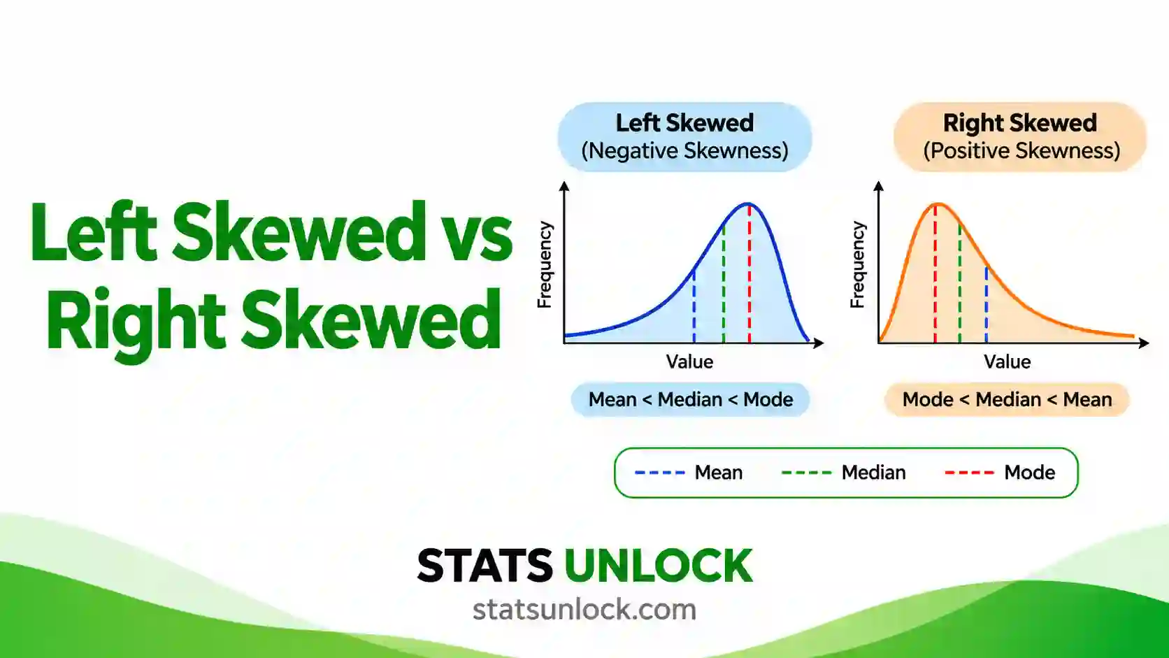
Left skewed vs right skewed describes which way the long tail of a distribution points: a left skewed (negative) distribution has its tail on the left and mean < median, while a right skewed (positive) distribution has its tail on the right and mean > median.
Skewness measures lopsidedness, not spread. Income, waiting times and hospital stays are usually right skewed. Easy exam scores, age at death and 5-star ratings are usually left skewed. Skewness does not tell you about outliers on its own, or about two peaks, so always look at a histogram or box plot as well.
Rule of thumb: G1 below −0.5 is left skewed, above +0.5 is right skewed, and between −0.5 and +0.5 is approximately symmetric. Beyond ±1 the skew is high. For example, hard exam scores give G1 = 1.72 (right skewed) and easy exam scores give G1 = −1.63 (left skewed).
Key takeaways
- Left skewed vs right skewed is about the tail: the side with the long, thin tail names the skew, not the side with the peak.
- In right skewed data the mean is usually above the median (here 50.35 vs 44.50); in left skewed data it is usually below (86.25 vs 90.00).
- Skewness between −0.5 and +0.5 is approximately symmetric, 0.5 to 1 in size is moderate, and above 1 is high.
- A skew is statistically real when the D’Agostino test gives p < 0.05, which needs n ≥ 8 and is stable from about n = 20.
- On a box plot the long whisker shows the skew; on a normal probability plot right skew bends up at the right and left skew bends down at the left.
📚 1. What Is Left Skewed vs Right Skewed?
Skewness measures how asymmetric a distribution is. A symmetric distribution looks the same on both sides of its centre, like a bell curve. A skewed distribution has one side that stretches out further than the other. That stretched side is called the tail, and the tail gives the skew its name.
- Right skewed (also called positively skewed or skewed to the right): most values sit on the low side and a few large values make a long tail to the right. Skewness is greater than 0.
- Left skewed (also called negatively skewed or skewed to the left): most values sit on the high side and a few small values make a long tail to the left. Skewness is less than 0.
- Symmetric: both tails are about the same length. Skewness is close to 0, and the mean, median and mode are close together.
What it actually measures. The moment skewness cubes each value’s distance from the mean. Cubing keeps the sign and makes far-away values count much more. So values far above the mean push the total up (right skew), and values far below the mean push it down (left skew). The result is divided by the standard deviation cubed, so skewness has no units. You can compare the skewness of exam scores with the skewness of incomes.
A worked one-liner: the hard exam scores 35, 36, 37, … 71, 88, 95 (n = 20) have mean 50.35 and median 44.50. The two scores of 88 and 95 drag the mean to the right. The adjusted skewness is G1 = 1.72, so these scores are highly right skewed.
A memory trick. Think of the tail as a pointing finger. If the long tail points to the right (toward larger numbers), the data are skewed right. If it points to the left (toward smaller numbers), the data are skewed left. Many students get this backwards because they look at where the hump is. The hump of a right skewed histogram sits on the left.
Who uses this: teachers check whether a test was too easy (left skew) or too hard (right skew). Economists report median income because income is right skewed. Clinicians report median length of stay. Ecologists see right skew in animal movement, body mass and species counts. Quality engineers watch for skew that signals a process drifting against a limit. Every analyst checks skewness before a t-test, ANOVA or regression, because strong skew can bias those tests.
| Feature | Left skewed (negative) | Symmetric | Right skewed (positive) |
|---|---|---|---|
| Long tail | Points left, toward small values | Both sides equal | Points right, toward large values |
| Skewness value | Below 0 (below −0.5 to matter) | About 0 (−0.5 to 0.5) | Above 0 (above 0.5 to matter) |
| Mean and median | Mean usually below median | Mean about equal to median | Mean usually above median |
| Usual order | mean < median < mode | mean = median = mode | mode < median < mean |
| Histogram | Peak on the right, bars trail off to the left | Bell shape | Peak on the left, bars trail off to the right |
| Box plot | Long left whisker, median near Q3 | Equal whiskers, median centred | Long right whisker, median near Q1 |
| Normal probability plot | Concave curve, bends down at the left | Straight line | Convex curve, bends up at the right |
| Typical examples | Easy test scores, age at death, star ratings | Adult height, measurement error | Income, house prices, waiting times |
| Usual fix | Reflect, then log; or rank-based tests | None needed | Log or square-root; or rank-based tests |
Skewness is not the same as kurtosis. Skewness asks “which side has the longer tail?”; kurtosis asks “how heavy are the tails overall?”. This tool reports both, but the verdict is based on skewness.
🧮 2. Set Up Your Data
Type or paste values separated by commas, for example 52, 48, 55, 61, 47. Spaces, tabs, semicolons and new lines also work, so a column copied from Excel is fine. Each box is one group (cluster).
Type one value per cell. Each column becomes a group, and you can rename the column headers. Empty cells are ignored, so groups can have different sizes.
📊 3. Results
🧠 4. Interpretation of Results, In Detail
4.1 Reading the verdict: which way is the skew?
Start with the sign of the skewness. A positive value means right skewed: the data have a long tail toward larger numbers. A negative value means left skewed: the long tail points toward smaller numbers. A value near zero means the two tails balance.
The name always follows the tail, never the peak. A right skewed histogram has its tallest bars on the left and thin bars trailing off to the right. That is why “skewed right vs skewed left” confuses so many students: the bulk of the data sits on the opposite side to the name. In the worked example, most hard-test scores are between 35 and 55, but two students scored 88 and 95. Those two scores form the right tail, so the hard test is right skewed.
4.2 How big is the skew? Reading the size of G1
The size (absolute value) of the skewness tells you how lopsided the data are. This tool uses the common rule of thumb associated with Bulmer:
- |G1| below 0.5: approximately symmetric. The mean is a fair summary.
- |G1| from 0.5 to 1: moderately skewed. Report the median as well as the mean.
- |G1| above 1: highly skewed. Lead with the median and IQR, and think about a transform before parametric tests.
Some textbooks are more lenient and treat values up to ±1, or even ±2, as acceptable for parametric tests (George and Mallery’s guideline). You can switch to the lenient bands in the settings. Whichever rule you use, name it in your methods so readers can judge.
4.3 Is the skew real? The standard error, z and the D’Agostino test
A sample can look skewed by chance, especially a small one. The standard error of skewness (SE) tells you how much skewness bounces around from sample to sample when the population is perfectly symmetric. For n = 20 it is 0.51, for n = 100 it is 0.24, and for n = 1000 it is 0.08.
Dividing G1 by its SE gives a z ratio. If |z| is above 1.96 the skew is significant at the 5% level. The D’Agostino skewness test refines this with a transformation that works well from n = 8 upward. It is the test behind scipy.stats.skewtest and R’s moments::agostino.test. A p-value below α means a sample this lopsided would be unusual if the population were symmetric.
Kim (2013) suggests a sample-size rule for the z ratio: use |z| > 1.96 below n = 50, |z| > 3.29 for n = 50 to 300, and judge the raw size of G1 (above 2 is substantial) for very large samples, where even trivial skew becomes significant.
4.4 Statistical significance vs practical importance
These two answer different questions. Significance asks “could this be chance?”; size asks “does it matter?”. With 600 values, a skew of 0.25 is significant (p = .012) but too small to change any decision. With 12 values, a skew of 1.1 can be non-significant even though the histogram is clearly lopsided. Always report both the size (G1) and the test (z and p), and let the size guide what you do.
4.5 The mean, median and mode: what they really tell you
The tail pulls the mean toward it, because the mean uses every value. The median barely moves. So in right skewed data the mean is usually above the median, and in left skewed data the mean is usually below it. That is why Pearson’s second coefficient, 3(mean − median) ÷ s, is a quick skewness check.
One warning: “mean > median means right skew” is a rule of thumb, not a law. Von Hippel (2005) showed it fails for many discrete distributions and for data with one long tail and one heavy short tail. When the mean-median order and G1 disagree, trust the histogram first, then G1, then the mean-median gap.
4.6 What the four charts show
Chart 1, the histogram. Bars left of the median are blue and bars right of the median are orange. The colour that stretches further marks the tail. The green curve is a normal distribution with the same mean and SD: where your bars rise above the curve on one side and fall below it on the other, you are seeing skew.
Chart 2, the box plot. In a right skewed box plot the right whisker is long and the median sits closer to Q1 (the left edge of the box). In a left skewed box plot the left whisker is long and the median sits closer to Q3. The orange diamond is the mean: it sits on the tail side of the median.
Chart 3, the normal probability (Q-Q) plot. Each point pairs a sorted data value with the value a normal distribution would predict. For right skewed data the points curve up and away from the line at the top right, a convex “smile”. For left skewed data they drop below the line at the bottom left, a concave “frown”.
Chart 4, skewness compared. Bars above zero are right skewed and below zero are left skewed. The green band is the symmetric zone. The black error bar on G1 is a rough 95% interval (G1 ± 1.96 SE): if it crosses zero, the skew may be chance.
4.7 Why three skewness coefficients disagree
G1, Pearson Sk2 and Bowley look at different parts of the data. G1 is driven by the cube of the distances, so it is dominated by the most extreme values. Pearson Sk2 compares the mean and median. Bowley uses only the quartiles, so it ignores the outer 25% on each side completely.
When G1 is large but Bowley is near zero, the middle half of your data is balanced and one or two extreme values create the skew. When all three agree in sign, the skew runs through the whole distribution. The pilot dataset in the samples shows the extreme case: G1 is +2.59 but Bowley is −0.50, because one value of 48 creates all of the positive skew.
4.8 Comparing two or more groups: left skewed vs right skewed side by side
When one group leans left and another leans right, as with the easy and hard tests, their means are misleading in opposite ways. The easy test mean (86.25) sits below its median (90.00), and the hard test mean (50.35) sits above its median (44.50). The gap in means is 35.90 points, but the gap in medians is 45.50 points. Comparing means understates how different the two classes really were.
For groups with opposite skew, compare medians, use a rank-based test such as Mann-Whitney or Kruskal-Wallis, or transform each group in a way that suits its own direction. Do not apply one log transform to both: it will make the left skewed group even more skewed.
4.9 Outliers, small samples and two peaks
Skewness is very sensitive to outliers. A single typing error, such as 950 instead of 95, can turn a symmetric sample into a highly skewed one. Check the outlier count in the checks table before trusting any verdict. With fewer than 20 values, removing or adding one point can flip the sign.
Two peaks are a different problem. A bimodal distribution can have skewness near zero and still look nothing like a bell curve. The tool reports the bimodality coefficient; values above 0.555 suggest two peaks (Pfister et al., 2013). Strong skew also pushes the coefficient up, so the tool only warns about two peaks when |G1| is below 0.75. If you see two humps in Chart 1, split the groups rather than describe one skewness.
4.10 Kurtosis, the companion number
Excess kurtosis (G2) describes how heavy both tails are compared with a normal curve. It is 0 for a normal distribution, positive when the tails are heavy, and negative when they are light. High skewness usually comes with positive kurtosis, because one heavy tail also raises tail weight. For a full kurtosis analysis use the leptokurtic vs platykurtic calculator listed in the related tools.
4.11 What skewness means for your next analysis
Mild skew (|G1| below 1) rarely harms t-tests or ANOVA once each group has 30 or more values, because the sampling distribution of the mean becomes close to normal. Strong skew with small groups is a problem: confidence intervals become lopsided and p-values become unreliable. In that case you can transform (log or square root for right skew; reflect then log for left skew), use a rank-based test, use a generalised linear model with a gamma or log-normal family, or bootstrap.
4.12 Common mistakes this calculator prevents
- Naming the skew after the peak instead of the tail.
- Mixing up G1 (Excel SKEW) and g1 (Excel SKEW.P, SciPy default) and reporting two different numbers for the same data.
- Calling a skew of 0.3 “skewed” because it is significant in a huge sample.
- Trusting the mean vs median order alone, which can mislead with discrete or bounded data.
- Forgetting that blanks, text or “n/a” codes in a column change n. The tool lists every ignored entry.
- Log-transforming left skewed data, which makes it worse.
✍ 5. How to Write Your Results in Research
Skewness usually appears in two places in a paper: the Methods, where you say how you checked distribution shape, and the Results, where you report the numbers. The five templates below fill in automatically after you run the analysis. Edit the wording to fit your study, but keep the numbers.
📌 Key conventions for this style
- Italicise statistical symbols in the final paper: G1, SE, z, p, M, Mdn, SD, n.
- Give p to two or three decimals with no leading zero (p = .003), and write p < .001 for very small values.
- Report skewness to two decimals, with its SE.
- Name the test: D’Agostino skewness test, or z = G1 / SE.
📌 Key conventions for this style
- Explain which skewness formula you used, because Excel, SPSS, R and Python give different values.
- State the threshold you used to call data skewed, and cite it.
- Say what you did about the skew: transform, rank-based test, or nothing, and why.
- Put the histograms or Q-Q plots in an appendix and refer to them.
📌 Key conventions for this style
- Avoid the word “skewness” and all symbols.
- Use “typical value” for the median and “average” for the mean.
- Describe the tail in words: “a few very large values”.
- Give units every time a number appears.
📌 Key conventions for this style
- Keep one line per group.
- Use square brackets for the IQR so it is not mistaken for a confidence interval.
- On a poster, show one small histogram per group next to the numbers.
- Keep decimals consistent across groups.
📌 Key conventions for this style
- Fix the threshold and the formula before you see the data.
- Say in advance what you will do if the skew passes the threshold.
- Record the quartile method (type 7 here) so Bowley skewness can be reproduced.
- Name the software and version.
5.1 Methods wording
Say three things in your methods: which skewness formula you used, how you judged it, and what you planned to do if data were skewed. For example: “Skewness was quantified with the adjusted Fisher-Pearson coefficient (G1; Joanes & Gill, 1998) and tested with the D’Agostino skewness test (D’Agostino et al., 1990). Distributions with |G1| ≥ 0.5 were treated as skewed; for these, medians and interquartile ranges are reported and group comparisons used the Mann-Whitney U test.”
5.2 The results sentence
Lead with the direction in words, then the numbers. Good: “Hard-test scores were right skewed (G1 = 1.72, SE = 0.51, z = 3.00, p = .003).” Weak: “Skewness was 1.722.” The weak version forces the reader to know that positive means right, and it gives no idea whether 1.722 is large or could be chance.
For two groups with opposite skew, put them in one sentence so the contrast is clear: “Easy-test scores were left skewed (G1 = −1.63, p = .004) whereas hard-test scores were right skewed (G1 = 1.72, p = .003).”
5.3 Tables and figures
In a descriptive table, add a column for skewness and, if space allows, its SE. Report mean (SD) for symmetric variables and median [IQR] for skewed ones, and say which is which in a footnote. For figures, a histogram or a box plot with raw points shows skew far better than a bar chart of means. Weissgerber et al. (2015) showed that bar graphs of means hide exactly the shape problems that skewness describes.
5.4 The discussion sentence
Explain what the skew means in your field. For example: “The left skew in easy-test scores reflects a ceiling effect: many students reached the maximum, so the test could not separate the strongest students.” Or: “Right skew in length of stay is driven by a small number of complicated cases, which matters for bed planning because the mean overstates the typical stay.”
5.5 Reporting checklist
- ✓ Direction in words: left skewed, right skewed or approximately symmetric.
- ✓ The coefficient with its name (G1, g1 or b1) and two decimals.
- ✓ The SE, z or the D’Agostino p-value, and n.
- ✓ Mean and median, so the reader sees the gap.
- ✓ The threshold you used and its source.
- ✓ What you did about it: transformation, non-parametric test, or a reason to do nothing.
- ✓ A histogram, box plot or Q-Q plot in the paper or supplement.
∑ 6. Formulas Used
These are the exact formulas this left skewed vs right skewed calculator uses. Every card ends with the worked numbers for the hard-test scores, so you can check each step by hand.
🔀 7. Skewness Calculation Flowchart, Step by Step
This flowchart shows how to decide left skewed vs right skewed, step by step, from a raw column of numbers to a tested verdict. Every box uses the same worked example as the Excel, R and Python sections: the 20 hard-test scores (35, 36, 37, 38, 39, 40, 41, 42, 43, 44, 45, 47, 48, 50, 51, 55, 62, 71, 88, 95). The easy-test totals are given in the final box.
Check any box yourself: the Excel sheet in Section 9, the R script in Section 10 and the Python script in Section 11 all return G1 = 1.7220, g1 = 1.5901, SE = 0.5121 and Z = 3.0036 for the hard test, and G1 = −1.6308 for the easy test.
📝 8. How to Use This Calculator
- Enter your data. In the Paste / Type tab, type or paste comma-separated numbers into a group box, for example 52, 48, 55, 61, 47. New lines, tabs and spaces also work.
- Name each group. Click the group name above each box and type a meaningful name such as Easy test. The name flows into the results table, all four charts and the report.
- Add more groups to compare. Press Add group to compare left skewed vs right skewed groups side by side. Each box has its own Clear and Remove button.
- Or upload a CSV or Excel file. On the Upload tab choose a file, then click the columns you want. Every selected column is loaded as its own group.
- Or type into the manual table. On the Manual Entry tab, each column is a group. Rename the headers, add rows or columns, then press Use this table.
- Try a sample dataset. Ten built-in datasets cover right skew (income, waiting time), left skew (easy tests, age at death, ratings), symmetric data and a messy pilot study.
- Choose your settings. Pick the skewness formula (G1 matches Excel SKEW), the size bands, the significance level, the histogram bins, decimals and units.
- Press Run Analysis. Nothing is calculated until you press the button, and changing any input clears old results so you never read stale numbers.
- Read the verdict and checks. Each group gets a coloured verdict card, the coefficients, the D’Agostino test and a list of data checks such as outliers and small samples.
- Use the charts and export. Read the histogram, box plot, normal probability plot and skewness chart, copy a reporting template from Section 5, and download the Doc or PDF report.
📈 9. How to Calculate Skewness in Excel (Left vs Right Skewed)
Excel can tell you whether data are left skewed or right skewed with one function, SKEW. What trips people up is everything around it: Excel has two skewness functions that give different numbers, it has no built-in p-value for skewness, and the Analysis ToolPak reports skewness without a standard error. This section shows each step on the hard-test scores with the spreadsheet on screen.
=SKEW(A2:A21) and press Enter. A positive answer means right skewed, a negative answer means left skewed. The hard test gives 1.7220.9.1 The functions you need
| You want | Excel function | Note |
|---|---|---|
| Skewness, adjusted G1 | =SKEW(A2:A21) | Matches SPSS, SAS, pandas and this tool’s default |
| Skewness, moment g1 | =SKEW.P(A2:A21) | Matches SciPy’s default and R moments::skewness. Excel 2013 and later |
| Excess kurtosis | =KURT(A2:A21) | 0 for a normal curve |
| Mean and median | =AVERAGE(A2:A21), =MEDIAN(A2:A21) | Mean above median hints right skew |
| Sample SD | =STDEV.S(A2:A21) | Use .S, not .P, for Pearson’s coefficient |
| Quartiles | =QUARTILE.INC(A2:A21,1) | Same method as R type 7 and NumPy |
| Count of numbers | =COUNT(A2:A21) | Use COUNT, not COUNTA, which counts text too |
| Normal tail area | =NORM.S.DIST(z,TRUE) | Turns a z value into a p-value |
| ToolPak summary | Data → Data Analysis → Descriptive Statistics | Reports SKEW and KURT. The Analysis ToolPak must be enabled first under File → Options → Add-ins |
9.2 Step by step
1 Put each group in its own column
Type a name in row 1 and the values underneath. Here the easy test is in column A and the hard test in column B, 20 scores each. Keep blanks blank; never type 0 for a missing value.
Easy test in A2:A21, hard test in B2:B21. Only the first eight rows are shown. The steps below copy the hard test into column A of a new sheet.
2 Get n, the mean and the median first
=COUNT(A2:A21)=AVERAGE(A2:A21)=MEDIAN(A2:A21)=STDEV.S(A2:A21)Putting the mean beside the median is the free first check: a mean well above the median points to a right tail.
n = 20, mean 50.35 in C3, median 44.5 in C4, SD 16.7026. The mean is 5.85 points above the median, the first sign of right skew.
3 Calculate skewness with SKEW, then the SE and z
=SKEW(A2:A21)=SKEW.P(A2:A21)=SQRT(6*20*19/(18*21*23))=C2/C4SKEW gives G1, SKEW.P gives g1. The third formula is the standard error for n = 20; replace the 20, 19, 18, 21 and 23 with n, n − 1, n − 2, n + 1 and n + 3 for your data.
SKEW = 1.7220, SKEW.P = 1.5901, SE = 0.5121, z = 3.3627. The p in C6 comes from =2*(1-NORM.S.DIST(ABS(C5),TRUE)).
4 Run the D’Agostino skewness test in eight cells
=SKEW.P(A2:A21)*SQRT((C2+1)*(C2+3)/(6*(C2-2)))=3*(C2^2+27*C2-70)*(C2+1)*(C2+3)/((C2-2)*(C2+5)*(C2+7)*(C2+9))=SQRT(2*(C4-1))-1=1/SQRT(LN(SQRT(C5)))=SQRT(2/(C5-1))=C6*ASINH(C3/C7)=2*(1-NORM.S.DIST(ABS(C8),TRUE))Put =COUNT(A2:A21) in C2, then the seven formulas above in C3 to C9 in that order. ASINH is Excel’s shortcut for ln[y + √(y² + 1)].
Y = 3.3627, β₂ = 3.5778, W² = 1.2706, δ = 2.8899, α = 2.7187, Z = 3.0036 in C8 and p = 0.0027 in C9, identical to R and Python.
5 Add the robust quartile skewness
=QUARTILE.INC(A2:A21,1)=(C4+C2-2*C3)/(C4-C2)=3*(AVERAGE(A2:A21)-MEDIAN(A2:A21))/STDEV.S(A2:A21)Bowley skewness only uses the quartiles, so it tells you whether the middle half of the data is lopsided too.
Q1 = 39.75, median 44.5, Q3 = 52, Bowley = 0.2245, Pearson Sk2 = 1.0507, KURT = 2.3861. All positive, so the right skew runs through the whole distribution.
9.3 The awkward cases
Excel gives skewness but no p-value. Neither SKEW nor the ToolPak tests it. Use the z ratio from step 3 for a quick answer, or the eight-cell D’Agostino chain from step 4 for the proper test. The quick z ratio is a little too generous in small samples: for the hard test it gives p = 0.0008, while the D’Agostino test gives 0.0027.
SKEW or SKEW.P? SKEW is the sample statistic most journals and SPSS users expect. SKEW.P treats your data as the whole population. For n = 20 they differ by about 8%; for n = 200 by under 1%.
Fewer than 3 values. SKEW returns #DIV/0! with fewer than three numbers or when every value is the same. That is correct: skewness is undefined there.
9.4 Why your Excel answer might differ from R or Python
| Situation | What happens | Fix |
|---|---|---|
Python scipy.stats.skew(x) | Gives g1 (1.5901), not Excel’s SKEW (1.7220) | Use skew(x, bias=False), or compare with SKEW.P |
R e1071::skewness(x) | Default type 3 gives b1 (1.4723) | Use type = 2 to match Excel SKEW |
R moments::skewness(x) | Gives g1 (1.5901) | Compare with SKEW.P, or adjust by √[n(n − 1)] ÷ (n − 2) |
pandas Series.skew() | Gives G1 (1.7220), same as Excel | No fix needed |
| p from the z ratio vs D’Agostino | 0.0008 vs 0.0027 for the hard test | They are different tests. Report which one you used |
SciPy skewtest on perfectly symmetric data | Returns z = 1.04 when g1 is exactly 0, because SciPy replaces y = 0 with 1 | Treat it as z = 0. R and this tool return 0 |
| Blank cells or text in the range | Excel skips them, so n is smaller than you think | Check COUNT first |
| Quartiles differ for Bowley | QUARTILE.EXC and SPSS use a different method | Use QUARTILE.INC, which matches R type 7 and NumPy |
| Tool | G1 (adjusted) | g1 (moment) | Skewness test |
|---|---|---|---|
| Excel | =SKEW(rng) | =SKEW.P(rng) | Build it, step 4 |
| Google Sheets | =SKEW(rng) | =SKEW.P(rng) | Same cell chain |
| R | e1071::skewness(x, type = 2) | moments::skewness(x) | moments::agostino.test(x) |
| Python SciPy | skew(x, bias=False) | skew(x) | skewtest(x) |
| Python pandas | s.skew() | not built in | use SciPy |
| SPSS | Analyze → Descriptive Statistics → Explore gives skewness (G1) with its standard error | ||
9.5 Making a left vs right skewed histogram and box plot in Excel
- Select one column of values, then Insert → Charts → Statistic → Histogram (Excel 2016 and later).
- Right-click the horizontal axis, choose Format Axis, and set a bin width that gives 5 to 10 bars. Too many bars hide the tail.
- For a box plot select both columns, then Insert → Statistic → Box and Whisker. Excel draws the mean as an ×; it sits on the tail side of the median line.
- Add the skewness to the chart title, for example “Hard test, G1 = 1.72”, so readers do not have to guess.
- Set the gap width to 0% on a histogram so the bars touch, which is what reviewers expect.
Charts 1 and 2 in Section 3 draw both plots for every group automatically, with the mean, median and fences marked.
9.6 Excel errors you will probably hit
| Excel shows | Why | Fix |
|---|---|---|
#DIV/0! from SKEW | Fewer than 3 numbers, or every value identical | Check COUNT and that the values vary |
#NAME? from SKEW.P | Excel 2010 or older | Use =SKEW(rng)*(n-2)/SQRT(n*(n-1)) |
#NUM! in the D’Agostino chain | n is below 8, so LN gets a non-positive value | The test needs n ≥ 8 |
#VALUE! | Text or units typed in a cell | Keep units in the header only |
| Skewness flips sign after an edit | One extreme value dominates a small sample | Check outliers; report Bowley as well |
| Green triangles in cell corners | Numbers stored as text and skipped | Select the column, click the warning icon, Convert to Number |
📈 10. How to Calculate Skewness in R (Left vs Right Skewed)
R has no skewness function in base R, so people install a package and are then surprised that e1071, moments and psych give three different numbers. The script below needs no packages. It computes G1 (Excel SKEW), g1, the standard error, the D’Agostino test, Pearson and Bowley skewness for every group, prints a plain-English verdict, and saves one publication-ready figure at 300 dpi with histograms, box plots and a normal probability plot.
Rscript. Change only the groups <- list(...) lines to use your own data.10.1 The complete script
R, base only, saves skewness_plot.png
# ============================================================
# Left skewed vs right skewed: skewness, D'Agostino test and
# one publication-ready figure (histograms, box plot, Q-Q plot)
# StatsUnlock - https://statsunlock.com/left-skewed-vs-right-skewed/
# Base R only. No packages to install.
# ============================================================

# ---- 1. Your data -------------------------------------------
# Replace with your own groups, or read a CSV:
#   df <- read.csv("data.csv")
#   groups <- list("Easy test" = na.omit(df$easy), "Hard test" = na.omit(df$hard))
groups <- list(
  "Easy test" = c(95, 92, 88, 97, 90, 85, 93, 78, 96, 89,
                  62, 91, 94, 87, 70, 98, 90, 83, 55, 92),
  "Hard test" = c(42, 48, 35, 51, 38, 62, 45, 40, 88, 37,
                  44, 55, 39, 47, 71, 36, 43, 50, 95, 41)
)
alpha <- 0.05
units <- "%"

# ---- 2. Skewness functions ----------------------------------
skew_g1 <- function(x) {                 # moment skewness = Excel SKEW.P
  d <- x - mean(x)
  mean(d^3) / mean(d^2)^1.5
}
skew_G1 <- function(x) {                 # adjusted = Excel SKEW, SPSS, SAS
  n <- length(x)
  skew_g1(x) * sqrt(n * (n - 1)) / (n - 2)
}
se_skew <- function(n) sqrt(6 * n * (n - 1) / ((n - 2) * (n + 1) * (n + 3)))
dagostino <- function(x) {               # same as moments::agostino.test
  n <- length(x)
  if (n < 8) return(c(Z = NA, p = NA))
  y  <- skew_g1(x) * sqrt((n + 1) * (n + 3) / (6 * (n - 2)))
  b2 <- 3 * (n^2 + 27 * n - 70) * (n + 1) * (n + 3) /
        ((n - 2) * (n + 5) * (n + 7) * (n + 9))
  w2 <- -1 + sqrt(2 * (b2 - 1))
  delta <- 1 / sqrt(log(sqrt(w2)))
  a  <- sqrt(2 / (w2 - 1))
  Z  <- delta * log(y / a + sqrt((y / a)^2 + 1))
  c(Z = Z, p = 2 * pnorm(-abs(Z)))
}

# ---- 3. Results for every group -----------------------------
res <- lapply(groups, function(x) {
  x  <- x[!is.na(x)]                     # drop missing values
  n  <- length(x)
  q  <- quantile(x, c(0.25, 0.5, 0.75))  # type 7, same as Excel
  G1 <- skew_G1(x)
  dz <- dagostino(x)
  list(n = n, mean = mean(x), median = median(x), sd = sd(x),
       g1 = skew_g1(x), G1 = G1, se = se_skew(n), z = G1 / se_skew(n),
       Z = unname(dz["Z"]), p = unname(dz["p"]),
       pearson2 = 3 * (mean(x) - median(x)) / sd(x),
       bowley = unname((q[3] + q[1] - 2 * q[2]) / (q[3] - q[1])))
})

for (nm in names(res)) {
  r <- res[[nm]]
  shape <- if (abs(r$G1) < 0.5) "approximately symmetric" else
    paste(if (abs(r$G1) > 1) "highly" else "moderately",
          if (r$G1 > 0) "right skewed (positive)" else "left skewed (negative)")
  sig <- if (!is.na(r$p) && r$p < alpha) "significant" else "not significant"
  cat(sprintf("\n%s  (n = %d)\n", nm, r$n))
  cat(sprintf("  mean = %.4f   median = %.4f   SD = %.4f\n", r$mean, r$median, r$sd))
  cat(sprintf("  G1 = %.4f   g1 = %.4f   SE = %.4f   z = %.4f\n", r$G1, r$g1, r$se, r$z))
  cat(sprintf("  D'Agostino Z = %.4f   p = %.4f\n", r$Z, r$p))
  cat(sprintf("  Pearson Sk2 = %.4f   Bowley = %.4f\n", r$pearson2, r$bowley))
  cat(sprintf("  Verdict: %s, %s at alpha = %.2f\n", shape, sig, alpha))
}

# ---- 4. One figure, four panels -----------------------------
cols <- c("#2563eb", "#ea580c", "#16a34a", "#9333ea")
png("skewness_plot.png", width = 3000, height = 2250, res = 300)
par(mfrow = c(2, 2), mar = c(4.5, 4.5, 3, 1), family = "sans")

for (k in 1:2) {                         # panels 1 and 2: histograms
  x <- groups[[k]]; r <- res[[k]]
  hist(x, breaks = "Sturges", col = adjustcolor(cols[k], 0.35), border = cols[k],
       main = sprintf("%s: G1 = %.2f, p = %.3f", names(groups)[k], r$G1, r$p),
       xlab = sprintf("Value (%s)", units), ylab = "Frequency", las = 1, cex.main = 1)
  abline(v = r$mean,   col = "#c2410c", lwd = 2.4, lty = 2)
  abline(v = r$median, col = "#9333ea", lwd = 2.4)
  legend(if (r$G1 < 0) "topleft" else "topright", bty = "n", cex = 0.85, lwd = 2.4, lty = c(2, 1),
         col = c("#c2410c", "#9333ea"),
         legend = c(sprintf("Mean %.2f", r$mean), sprintf("Median %.2f", r$median)))
}

boxplot(groups, horizontal = TRUE, outline = FALSE, las = 1, col = "white",
        main = "Box plot: long whisker = tail side", cex.main = 1,
        xlab = sprintf("Value (%s)", units),
        ylim = range(unlist(groups)))
set.seed(42)                             # seed = reproducible jitter
for (k in seq_along(groups)) {
  x <- groups[[k]]
  points(x, k + runif(length(x), -0.15, 0.15), pch = 19,
         col = adjustcolor(cols[k], 0.6))
  points(res[[k]]$mean, k, pch = 23, bg = "#c2410c", col = "#c2410c", cex = 1.6)
}

qq <- lapply(groups, qqnorm, plot.it = FALSE)
plot(NULL, xlim = range(sapply(qq, function(q) range(q$x))),
     ylim = range(unlist(groups)), las = 1, main = "Normal probability plot",
     cex.main = 1, xlab = "Theoretical normal quantile",
     ylab = sprintf("Sample value (%s)", units))
for (k in seq_along(groups)) {
  points(qq[[k]]$x, qq[[k]]$y, pch = 19, col = cols[k])
  qqline(groups[[k]], col = cols[k], lty = 2)
}
legend("topleft", bty = "n", pch = 19, col = cols[seq_along(groups)],
       legend = names(groups), cex = 0.85)

dev.off()
cat("\nSaved skewness_plot.png\n")
Run it with Rscript skewness.R. It prints G1 = −1.6308 (Z = −2.8827, p = 0.0039) for the easy test and G1 = 1.7220 (Z = 3.0036, p = 0.0027) for the hard test, matching Excel and Python.
10.2 What each part does
| Line or function | What it does, and why it is there |
|---|---|
| groups <- list(...) | One named vector per group. The names become panel titles and labels. na.omit() in the CSV line drops missing values so n is honest. |
| skew_g1() | The moment skewness: the mean of the cubed deviations divided by the variance (divisor n) to the power 1.5. Same as Excel SKEW.P and moments::skewness. |
| skew_G1() | Multiplies g1 by √[n(n − 1)] ÷ (n − 2). This is Excel SKEW, SPSS, SAS and e1071::skewness(x, type = 2). |
| se_skew() | The standard error of G1. It depends only on n, not on the data. |
| dagostino() | The D’Agostino (1970) skewness test, written out so you can see every constant. It returns the same Z and p as moments::agostino.test(). It returns NA when n < 8. |
| quantile(x, c(.25,.5,.75)) | Quartiles with R’s default type 7, identical to Excel QUARTILE.INC and NumPy. Needed for Bowley skewness. |
| lapply(groups, ...) | Runs the same calculations on every group and returns a list of results, one per group. |
| if (abs(r$G1) < 0.5) | The size rule: below 0.5 symmetric, 0.5 to 1 moderate, above 1 high. Change 0.5 and 1 to 1 and 2 for the lenient rule. |
| png(..., res = 300) | Opens a 300 dpi file. Without res you get a blurry 72 dpi image that journals reject. |
| par(mfrow = c(2, 2)) | Splits the figure into a 2 by 2 grid of panels. |
| hist(..., breaks = "Sturges") | Draws each histogram with Sturges bins, the same default as this tool, so the shapes match Chart 1. |
| boxplot(..., horizontal = TRUE, outline = FALSE) | Horizontal box plots, so “right skewed” really points right. outline = FALSE stops outliers being drawn twice, because every point is added next. |
| set.seed(42) | Fixes the random vertical jitter so the figure is reproducible. |
| qqnorm(..., plot.it = FALSE), qqline() | Computes the normal probability plot points without drawing, so both groups can share one panel, then adds a reference line through the quartiles. |
| dev.off() | Closes the file. Forgetting it leaves an empty or locked PNG, the most common R plotting error. |
10.3 What the figure shows
The top two panels are histograms. The easy test piles up near 90 to 100 with a few low scores trailing left: the mean line (dashed) sits left of the median line, the picture of left skew. The hard test piles up near 40 with a tail running right to 95: the mean sits right of the median, the picture of right skew.
The bottom left panel puts the two box plots on one scale. The easy test has its long whisker and loose points on the left; the hard test has them on the right. The bottom right panel is the normal probability plot: the hard-test points bend up away from their line at the right end (convex), and the easy-test points bend down away from their line at the left end (concave).
10.4 Common R problems and fixes
| Symptom | Cause | Fix |
|---|---|---|
could not find function "skewness" | Base R has none | Use the functions in the script, or library(moments) |
| e1071 and Excel disagree | e1071 defaults to type 3 (b1) | e1071::skewness(x, type = 2) |
| moments and SPSS disagree | moments returns g1, SPSS returns G1 | Use skew_G1() from the script |
Result is NA | A missing value in the vector | x <- x[!is.na(x)] before calculating |
agostino.test error about sample size | n is below 8 | Report G1 and SE only |
| The PNG is empty | dev.off() never ran | Run while (dev.cur() > 1) dev.off() |
| Legend covers the bars | Tail and legend on the same side | The script already moves it; change "topleft" if needed |
10.5 Useful one-liners
| You want | R code |
|---|---|
| G1, Excel SKEW | e1071::skewness(x, type = 2) |
| g1, Excel SKEW.P | moments::skewness(x) |
| D’Agostino test | moments::agostino.test(x) |
| Skewness by group | tapply(df$value, df$group, function(v) e1071::skewness(v, type = 2)) |
| Quick normal probability plot | qqnorm(x); qqline(x) |
| Log transform for right skew | skew_G1(log(x)) |
| Reflect, then log, for left skew | skew_G1(log(max(x) + 1 - x)) |
| Bootstrap 95% CI for G1 | quantile(replicate(5000, skew_G1(sample(x, replace = TRUE))), c(.025, .975)) |
📈 11. How to Calculate Skewness in Python (Left vs Right Skewed)
In Python, scipy.stats.skew(x) is one line, but its default is the moment estimate g1, which disagrees with Excel, SPSS and pandas. The script below computes both, runs the D’Agostino test with scipy.stats.skewtest, prints a verdict for each group, and saves one 300 dpi figure with histograms, box plots and a normal probability plot.
groups = {...} lines. It runs in a terminal, VS Code, Spyder or Jupyter.Install with pip install numpy scipy matplotlib if you do not already have them. Add pandas only if you use the CSV line.
11.1 The complete script
Python 3, saves skewness_plot.png
# ============================================================
# Left skewed vs right skewed: skewness, D'Agostino test and
# one publication-ready figure (histograms, box plot, Q-Q plot)
# StatsUnlock - https://statsunlock.com/left-skewed-vs-right-skewed/
# ============================================================
import numpy as np
from scipy import stats
import matplotlib
matplotlib.use("Agg")                     # draw to file, no window needed
import matplotlib.pyplot as plt

# ---- 1. Your data -------------------------------------------
# Replace with your own groups, or read a CSV:
#   import pandas as pd
#   df = pd.read_csv("data.csv")
#   groups = {c: df[c].dropna().to_numpy(float) for c in ["Easy test", "Hard test"]}
groups = {
    "Easy test": np.array([95, 92, 88, 97, 90, 85, 93, 78, 96, 89,
                           62, 91, 94, 87, 70, 98, 90, 83, 55, 92], dtype=float),
    "Hard test": np.array([42, 48, 35, 51, 38, 62, 45, 40, 88, 37,
                           44, 55, 39, 47, 71, 36, 43, 50, 95, 41], dtype=float),
}
alpha = 0.05
units = "%"

# ---- 2. Skewness for every group ----------------------------
def skew_report(x):
    x = x[~np.isnan(x)]                   # drop missing values
    n = len(x)
    g1 = stats.skew(x)                    # moment skewness = Excel SKEW.P
    G1 = stats.skew(x, bias=False)        # adjusted = Excel SKEW, SPSS, SAS
    se = np.sqrt(6 * n * (n - 1) / ((n - 2) * (n + 1) * (n + 3)))
    q1, med, q3 = np.percentile(x, [25, 50, 75])   # type 7, same as Excel
    out = dict(n=n, mean=x.mean(), median=med, sd=x.std(ddof=1),
               g1=g1, G1=G1, se=se, z=G1 / se,
               pearson2=3 * (x.mean() - med) / x.std(ddof=1),
               bowley=(q3 + q1 - 2 * med) / (q3 - q1),
               kurt=stats.kurtosis(x, bias=False))  # = Excel KURT
    if n >= 8:
        out["Z"], out["p"] = stats.skewtest(x)       # D'Agostino test
    else:
        out["Z"], out["p"] = np.nan, np.nan
    return out

results = {name: skew_report(x) for name, x in groups.items()}

for name, r in results.items():
    if abs(r["G1"]) < 0.5:
        shape = "approximately symmetric"
    else:
        size = "highly" if abs(r["G1"]) > 1 else "moderately"
        side = "right skewed (positive)" if r["G1"] > 0 else "left skewed (negative)"
        shape = f"{size} {side}"
    sig = "significant" if r["p"] < alpha else "not significant"
    print(f"\n{name}  (n = {r['n']})")
    print(f"  mean = {r['mean']:.4f}   median = {r['median']:.4f}   SD = {r['sd']:.4f}")
    print(f"  G1 = {r['G1']:.4f}   g1 = {r['g1']:.4f}   SE = {r['se']:.4f}   z = {r['z']:.4f}")
    print(f"  D'Agostino Z = {r['Z']:.4f}   p = {r['p']:.4f}")
    print(f"  Pearson Sk2 = {r['pearson2']:.4f}   Bowley = {r['bowley']:.4f}   kurtosis = {r['kurt']:.4f}")
    print(f"  Verdict: {shape}, {sig} at alpha = {alpha}")

# ---- 3. One figure, four panels -----------------------------
colors = ["#2563eb", "#ea580c", "#16a34a", "#9333ea"]
names = list(groups)
fig, ax = plt.subplots(2, 2, figsize=(10, 7.5))
rng = np.random.default_rng(42)           # seed = reproducible jitter

for k, name in enumerate(names[:2]):      # panels 1 and 2: histograms
    x, r, a = groups[name], results[name], ax[0, k]
    a.hist(x, bins="sturges", color=colors[k], alpha=0.35, edgecolor=colors[k])
    a.axvline(r["mean"], color="#c2410c", ls="--", lw=2, label=f"Mean {r['mean']:.2f}")
    a.axvline(r["median"], color="#9333ea", lw=2, label=f"Median {r['median']:.2f}")
    a.set_title(f"{name}: G1 = {r['G1']:.2f}, p = {r['p']:.3f}", fontsize=11, loc="left")
    a.set_xlabel(f"Value ({units})")
    a.set_ylabel("Frequency")
    a.legend(frameon=False, fontsize=9)

a = ax[1, 0]                              # panel 3: box plots with points
box_kw = dict(widths=0.5, showfliers=False, medianprops=dict(color="black", lw=2))
try:
    a.boxplot([groups[n] for n in names], orientation="horizontal", **box_kw)
except TypeError:                         # Matplotlib older than 3.10
    a.boxplot([groups[n] for n in names], vert=False, **box_kw)
for k, name in enumerate(names):
    x = groups[name]
    a.scatter(x, k + 1 + rng.uniform(-0.15, 0.15, len(x)),
              color=colors[k % 4], alpha=0.6, s=18, zorder=3)
    a.scatter(results[name]["mean"], k + 1, marker="D", color="#c2410c", s=50, zorder=4)
a.set_yticks(range(1, len(names) + 1))
a.set_yticklabels(names)
a.set_title("Box plot: long whisker = tail side", fontsize=11, loc="left")
a.set_xlabel(f"Value ({units})")

a = ax[1, 1]                              # panel 4: normal Q-Q plots
for k, name in enumerate(names):
    (osm, osr), (slope, icpt, _) = stats.probplot(groups[name], dist="norm")
    a.scatter(osm, osr, color=colors[k % 4], s=18, label=name)
    a.plot(osm, slope * osm + icpt, color=colors[k % 4], lw=1.2, ls="--")
a.set_title("Normal probability plot", fontsize=11, loc="left")
a.set_xlabel("Theoretical normal quantile")
a.set_ylabel(f"Sample value ({units})")
a.legend(frameon=False, fontsize=9)

fig.suptitle("Left skewed vs right skewed", fontsize=14, fontweight="bold")
fig.tight_layout()
fig.savefig("skewness_plot.png", dpi=300, bbox_inches="tight")
print("\nSaved skewness_plot.png")
Run it with python skewness.py. In Jupyter, delete the matplotlib.use("Agg") line and add plt.show() at the end to see the figure inline.
11.2 What each part does
| Line or function | What it does, and why it is there |
|---|---|
| dtype=float | Makes every array floating point so no integer arithmetic can creep in. |
| x[~np.isnan(x)] | Drops missing values. Without it, every statistic becomes nan. |
| stats.skew(x) | The moment skewness g1 (default bias=True). Matches Excel SKEW.P, not SKEW. |
| stats.skew(x, bias=False) | The adjusted G1. Matches Excel SKEW, SPSS, SAS and pandas.Series.skew(). |
| np.sqrt(6*n*(n-1)/...) | The standard error of skewness. SciPy does not report it, so it is computed here. |
| np.percentile(x, [25, 50, 75]) | Quartiles with the linear method, identical to Excel QUARTILE.INC and R type 7. |
| x.std(ddof=1) | The sample SD. NumPy’s default ddof=0 is the population SD and would not match Excel STDEV.S. |
| stats.kurtosis(x, bias=False) | Excess kurtosis matching Excel KURT. |
| stats.skewtest(x) | The D’Agostino skewness test. Needs n ≥ 8. One quirk: with skewness exactly 0 it returns z ≈ 1.04 instead of 0, because it replaces 0 with 1 internally. |
| matplotlib.use("Agg") | Draws straight to a file, so the script also works on servers with no screen. |
| default_rng(42) | A seeded random generator for the jitter, so the figure is reproducible. |
| boxplot(..., orientation=...) | Horizontal box plots. The try/except keeps it working on Matplotlib versions older than 3.10, which use vert=False. |
| stats.probplot(x, dist="norm") | Returns the normal probability plot points and a fitted line for each group. |
| savefig(..., dpi=300, bbox_inches="tight") | Saves at print quality and trims empty margins. |
11.3 What the figure shows
The four panels match the R figure. The histograms show the easy test leaning left and the hard test leaning right, with the mean line pulled toward each tail. The box plots put both groups on one axis so you can see the long whiskers on opposite sides. On the normal probability plot, the hard-test points curve upward at the right end and the easy-test points curve downward at the left end. Matplotlib picks slightly different histogram edges from R, so bar heights can differ, but every number printed is identical.
11.4 Common Python problems and fixes
| Symptom | Cause | Fix |
|---|---|---|
| SciPy gives 1.5901, Excel gives 1.7220 | SciPy defaults to g1 | stats.skew(x, bias=False) |
| pandas and SciPy disagree | pandas uses G1, SciPy uses g1 | Pass bias=False to SciPy |
Result is nan | Missing values in the array | x = x[~np.isnan(x)], or nan_policy="omit" |
skewtest warning about n | Fewer than 8 values | Report G1 and SE only |
| SD does not match Excel | NumPy uses ddof = 0 by default | x.std(ddof=1) |
| Figure is blank in Jupyter | The Agg backend draws only to file | Remove the matplotlib.use line and call plt.show() |
Deprecation warning about vert | Matplotlib 3.11 or later | The script already uses orientation first |
11.5 Useful one-liners
| You want | Python code |
|---|---|
| G1, Excel SKEW | stats.skew(x, bias=False) |
| g1, Excel SKEW.P | stats.skew(x) |
| Skewness of every column | df.skew(numeric_only=True) |
| Skewness by group | df.groupby("group")["value"].skew() |
| D’Agostino test | stats.skewtest(x) |
| Log transform for right skew | stats.skew(np.log(x), bias=False) |
| Reflect, then log, for left skew | stats.skew(np.log(x.max() + 1 - x), bias=False) |
| Box-Cox, finds the best power | y, lam = stats.boxcox(x) |
bias=False in Python, type = 2 in e1071, or SKEW vs SKEW.P in Excel.📋 12. Reference Tables
12.1 How to read the size of skewness
| |Skewness| | Standard rule (Bulmer) | Lenient rule (George & Mallery) | What to report |
|---|---|---|---|
| below 0.5 | Approximately symmetric | Acceptable | Mean and SD |
| 0.5 to 1 | Moderately skewed | Acceptable | Mean and SD plus median |
| 1 to 2 | Highly skewed | Moderate | Median and IQR first |
| above 2 | Highly skewed | High | Median and IQR; transform or rank-based test |
What to conclude: the sign gives the direction (positive = right, negative = left) and these bands give the size. Name the rule you used. Kim (2013) and Blanca et al. (2013) discuss why real data rarely have skewness exactly 0.
12.2 Left skewed vs right skewed vs symmetric at a glance
| Clue | Skewed left | Symmetric | Skewed right |
|---|---|---|---|
| Skewness sign | Negative | About 0 | Positive |
| Mean vs median | Mean < median (usually) | Mean ≈ median | Mean > median (usually) |
| Mean, median, mode order | Mean < median < mode | All equal | Mode < median < mean |
| Median − min vs max − median | Left gap longer | About equal | Right gap longer |
| Quartiles | Q2 − Q1 > Q3 − Q2 | Equal | Q3 − Q2 > Q2 − Q1 |
| Other names | Negatively skewed, skewed to the left | Normal-like, bell shaped | Positively skewed, skewed to the right |
What to conclude: if three or more clues point the same way, the direction is clear. If they disagree, look at the histogram and trust G1 over the mean-median order (von Hippel, 2005).
12.3 How skew looks in each graph
| Graph | Skewed left looks like | Skewed right looks like |
|---|---|---|
| Histogram | Tall bars on the right, short bars trailing left | Tall bars on the left, short bars trailing right |
| Box plot | Long left whisker; median nearer Q3; outliers on the left | Long right whisker; median nearer Q1; outliers on the right |
| Dot plot | Dots stacked high on the right, spread thinly to the left | Dots stacked high on the left, spread thinly to the right |
| Stem-and-leaf plot | Long leaves on the high stems, few leaves on the low stems | Long leaves on the low stems, few leaves on the high stems |
| Bar graph of frequencies | Bars rise toward the right category | Bars fall away toward the right category |
| Normal probability plot | Concave: points fall below the line at the left end | Convex: points rise above the line at the right end |
| Density curve | Peak on the right, tail to the left | Peak on the left, tail to the right |
What to conclude: in every graph the tail, the sparse side, names the skew. A stem-and-leaf plot is a histogram turned on its side, so read it the same way.
12.4 Standard error of skewness and the smallest significant |G1|
| n | SE of skewness | |G1| needed, α = 0.05 (1.96 × SE) | |G1| needed, α = 0.01 (2.576 × SE) | Note |
|---|---|---|---|---|
| 8 | 0.752 | 1.474 | 1.937 | Smallest n for the D’Agostino test |
| 10 | 0.687 | 1.347 | 1.770 | Very unstable |
| 15 | 0.580 | 1.137 | 1.494 | Unstable |
| 20 | 0.512 | 1.004 | 1.319 | Worked example size |
| 30 | 0.427 | 0.837 | 1.100 | Common minimum |
| 50 | 0.337 | 0.660 | 0.867 | Moderate |
| 100 | 0.241 | 0.473 | 0.622 | Good |
| 200 | 0.172 | 0.337 | 0.443 | Good |
| 500 | 0.109 | 0.214 | 0.281 | Large: tiny skew becomes significant |
| 1000 | 0.077 | 0.152 | 0.199 | Very large: judge size, not p |
What to conclude: with 20 values a skewness under about 1.00 can be chance; with 500 values even 0.21 is significant. That is why size matters more than p in large samples. These are z-ratio cut-offs; the D’Agostino test is slightly stricter in small samples.
12.5 Which software gives which skewness
| Formula | Hard-test value | Used by |
|---|---|---|
| G1, adjusted Fisher-Pearson | 1.7220 | Excel SKEW, SPSS, SAS, Stata (detail), pandas .skew(), SciPy bias=False, e1071 type 2, this tool’s default |
| g1, moment coefficient | 1.5901 | Excel SKEW.P, SciPy default, R moments::skewness, e1071 type 1 |
| b1 | 1.4723 | Minitab, R e1071 type 3 (its default), psych::skew |
What to conclude: the three always share the same sign, so they never disagree about left vs right. They only differ in size, by up to about 15% at n = 20 and under 1% at n = 1000 (Joanes & Gill, 1998).
12.6 Fixing skewed data before a parametric test
| Skew | Try first | Stronger option | No-transform option |
|---|---|---|---|
| Mild right (0.5 to 1) | Square root, √x | Log, ln(x + 1) if zeros | Welch t-test or ANOVA with n ≥ 30 per group |
| Strong right (above 1) | Log, ln(x) | Reciprocal 1/x, or Box-Cox | Mann-Whitney, Kruskal-Wallis, gamma GLM |
| Mild left (−0.5 to −1) | Square, x² | Reflect then √: √(max + 1 − x) | Rank-based tests |
| Strong left (below −1) | Reflect then log: ln(max + 1 − x) | Box-Cox on the reflected values | Rank-based tests, bootstrap the median |
What to conclude: never log-transform left skewed data directly; it stretches the left tail further. After reflecting, the direction of effects flips, so say so when you report results (Box & Cox, 1964; Feng et al., 2014).
12.7 Real-world variables and their usual skew
| Usually right skewed | Usually left skewed | Usually close to symmetric |
|---|---|---|
| Household income, wealth | Age at death in rich countries | Adult height within one sex |
| House prices | Scores on an easy test | Measurement error |
| Hospital length of stay | Product star ratings | Blood pressure in healthy adults |
| Reaction and waiting times | Gestational age at birth | IQ scores (by design) |
| Animal movement distances, body mass | Percentage of a task completed | Daily temperature at one site |
| Insurance claims, city sizes | Retirement age | Sums of many small effects |
What to conclude: a hard floor (zero, or a minimum) with no ceiling gives right skew; a hard ceiling (100%, 5 stars, a maximum lifespan) gives left skew. Micceri (1989) found most real psychological data are skewed to some degree.
📈 13. Example Results
Eight worked examples, from a clean textbook case to the situations that fool people. In every histogram, blue bars are below the median and orange bars are above it, the dashed line is the mean and the solid line is the median.
Skewed left vs skewed right, mirror images
Two groups that are exact reflections of each other.
A teaching set of 15 values on a 1 to 10 scale. The right skewed group is built by reflecting the left skewed group (11 − x), so the only thing that changes is the direction.
| Statistic | Value | Note |
|---|---|---|
| n | 15 | Values used |
| Mean | 3.2000 | Pulled toward the tail |
| Median | 3.0000 | Middle value |
| SD | 2.1778 | Sample, n − 1 |
| Skewness G1 | 1.4765 | Excel SKEW |
| Skewness g1 | 1.3245 | Excel SKEW.P |
| SE of skewness | 0.5801 | Depends only on n |
| z = G1 ÷ SE | 2.545 | |z| > 1.96 suggests real skew |
| D’Agostino Z | 2.4222 | Skewness test |
| D’Agostino p | 0.0154 | Two-sided |
| Pearson Sk2 | 0.2755 | 3(mean − median) ÷ s |
| Bowley | 0.0000 | Quartile skewness |
| Mirror group G1 | −1.4765 | Same size, opposite sign |
What it means: The skewed-right group has G1 = 1.4765 and the skewed-left group has G1 = −1.4765: exactly the same size with the opposite sign, because reflecting data flips the sign of skewness and nothing else. Both are highly skewed and both are significant (p = 0.0154). Note Bowley is 0 here because the quartiles sit evenly around the median; all the skew comes from the outer values.
How to write it: “Group R was right skewed (G1 = 1.48, SE = 0.58, p = .015) and its mirror, group L, was left skewed (G1 = −1.48).”
Household income is right skewed
The classic positively skewed variable.
Twenty household incomes in thousand USD from one neighbourhood survey.
| Statistic | Value | Note |
|---|---|---|
| n | 20 | Values used |
| Mean | 65.6000 | Pulled toward the tail |
| Median | 46.5000 | Middle value |
| SD | 49.3477 | Sample, n − 1 |
| Skewness G1 | 1.8589 | Excel SKEW |
| Skewness g1 | 1.7164 | Excel SKEW.P |
| SE of skewness | 0.5121 | Depends only on n |
| z = G1 ÷ SE | 3.630 | |z| > 1.96 suggests real skew |
| D’Agostino Z | 3.1780 | Skewness test |
| D’Agostino p | 0.0015 | Two-sided |
| Pearson Sk2 | 1.1611 | 3(mean − median) ÷ s |
| Bowley | 0.4110 | Quartile skewness |
What it means: G1 = 1.86 is well above 1, so income is highly right skewed, and the D’Agostino test is clearly significant (p = 0.0015). The mean (65.6) is 19.1 thousand above the median (46.5), so 13 of the 20 households earn less than the “average”. Report the median.
How to write it: “Household income was highly right skewed (G1 = 1.86, SE = 0.51, D’Agostino z = 3.18, p = .001); median income was 46.5 thousand USD (IQR 34.50 to 75.25).”
Moderate right skew that may be chance
Large enough to notice, not quite significant.
Twenty commute times in minutes recorded by one office.
| Statistic | Value | Note |
|---|---|---|
| n | 20 | Values used |
| Mean | 18.7500 | Pulled toward the tail |
| Median | 17.5000 | Middle value |
| SD | 5.7754 | Sample, n − 1 |
| Skewness G1 | 0.9443 | Excel SKEW |
| Skewness g1 | 0.8719 | Excel SKEW.P |
| SE of skewness | 0.5121 | Depends only on n |
| z = G1 ÷ SE | 1.844 | |z| > 1.96 suggests real skew |
| D’Agostino Z | 1.8344 | Skewness test |
| D’Agostino p | 0.0666 | Two-sided |
| Pearson Sk2 | 0.6493 | 3(mean − median) ÷ s |
| Bowley | 0.2000 | Quartile skewness |
What it means: G1 = 0.94 is in the moderate band (0.5 to 1), and the mean sits 1.25 minutes above the median. But the D’Agostino test gives p = 0.067, just above 0.05, so with only 20 values the skew could be sampling noise. Report it as moderate right skew that did not reach significance, and give both mean and median.
How to write it: “Commute time showed moderate positive skew (G1 = 0.94, SE = 0.51) that was not statistically significant (D’Agostino z = 1.83, p = .067).”
Adult height is close to symmetric
What “no skew” looks like.
Twenty adult heights in centimetres from one population.
| Statistic | Value | Note |
|---|---|---|
| n | 20 | Values used |
| Mean | 171.6000 | Pulled toward the tail |
| Median | 171.5000 | Middle value |
| SD | 6.6760 | Sample, n − 1 |
| Skewness G1 | 0.1324 | Excel SKEW |
| Skewness g1 | 0.1222 | Excel SKEW.P |
| SE of skewness | 0.5121 | Depends only on n |
| z = G1 ÷ SE | 0.258 | |z| > 1.96 suggests real skew |
| D’Agostino Z | 0.2743 | Skewness test |
| D’Agostino p | 0.7838 | Two-sided |
| Pearson Sk2 | 0.0449 | 3(mean − median) ÷ s |
| Bowley | 0.0000 | Quartile skewness |
What it means: G1 = 0.13 is far inside the ±0.5 band, the mean (171.60) and median (171.50) differ by 0.10 cm, and the test is nowhere near significant (p = 0.784). The data are approximately symmetric, so the mean and SD are a fair summary.
How to write it: “Height was approximately symmetric (G1 = 0.13, SE = 0.51, p = .784); M = 171.6 cm, SD = 6.7.”
A pilot study with only 7 values
Huge skewness, but too little data to trust it.
A pilot recorded nine entries: 12, 14, 13, n/a, 15, 11, a blank, 14 and 48. After dropping the blank and the n/a code, 7 values remain.
| Statistic | Value | Note |
|---|---|---|
| n | 7 | Values used |
| Mean | 18.1429 | Pulled toward the tail |
| Median | 14.0000 | Middle value |
| SD | 13.2342 | Sample, n − 1 |
| Skewness G1 | 2.5882 | Excel SKEW |
| Skewness g1 | 1.9969 | Excel SKEW.P |
| SE of skewness | 0.7937 | Depends only on n |
| z = G1 ÷ SE | 3.261 | |z| > 1.96 suggests real skew |
| D’Agostino Z | n/a | Skewness test |
| D’Agostino p | n < 8, test not run | Two-sided |
| Pearson Sk2 | 0.9391 | 3(mean − median) ÷ s |
| Bowley | −0.5000 | Quartile skewness |
What it means: G1 = 2.59 looks enormous, but it is created by a single value. The D’Agostino test needs at least 8 values, so it cannot run; the rough z ratio is 3.26. Bowley skewness is −0.50, the opposite sign, because the middle half is not right skewed at all. Check whether 48 is a typing error before saying anything about shape.
How to write it: “With n = 7, skewness (G1 = 2.59) was driven by a single extreme value and was not tested formally.”
Six hundred glucose readings
Significant does not mean important.
Six hundred fasting glucose readings in mg/dL from a screening programme.
| Statistic | Value | Note |
|---|---|---|
| n | 600 | Values used |
| Mean | 94.9991 | Pulled toward the tail |
| Median | 94.6650 | Middle value |
| SD | 7.7436 | Sample, n − 1 |
| Skewness G1 | 0.2530 | Excel SKEW |
| Skewness g1 | 0.2524 | Excel SKEW.P |
| SE of skewness | 0.0998 | Depends only on n |
| z = G1 ÷ SE | 2.537 | |z| > 1.96 suggests real skew |
| D’Agostino Z | 2.5169 | Skewness test |
| D’Agostino p | 0.0118 | Two-sided |
| Pearson Sk2 | 0.1294 | 3(mean − median) ÷ s |
| Bowley | 0.0298 | Quartile skewness |
What it means: G1 = 0.25 is small, inside the symmetric band, yet the test says p = 0.012. With 600 values the standard error is only 0.100, so even a trivial lean becomes significant. The mean and median differ by just 0.33 mg/dL. Treat these data as approximately symmetric and use the mean.
How to write it: “Glucose showed slight positive skew (G1 = 0.25, SE = 0.10, p = .012) that was statistically significant but too small to affect the analysis.”
Five-star ratings: skew from a ceiling
When the scale, not the people, makes the skew.
Twenty-five customer reviews on a 1 to 5 star scale. Fifteen are 5 stars.
| Statistic | Value | Note |
|---|---|---|
| n | 25 | Values used |
| Mean | 4.3200 | Pulled toward the tail |
| Median | 5.0000 | Middle value |
| SD | 1.0693 | Sample, n − 1 |
| Skewness G1 | −1.8212 | Excel SKEW |
| Skewness g1 | −1.7101 | Excel SKEW.P |
| SE of skewness | 0.4637 | Depends only on n |
| z = G1 ÷ SE | −3.928 | |z| > 1.96 suggests real skew |
| D’Agostino Z | −3.3627 | Skewness test |
| D’Agostino p | 0.0008 | Two-sided |
| Pearson Sk2 | −1.9078 | 3(mean − median) ÷ s |
| Bowley | −1.0000 | Quartile skewness |
What it means: G1 = −1.82 says highly left skewed and p = 0.0008, but the median equals Q3 (both 5), so Bowley hits its limit of −1. Skewness here mostly describes the ceiling of the scale. With so few distinct values, report the percentage of 5-star ratings and the median, and use rank-based tests rather than a t-test.
How to write it: “Ratings were bounded at the top of the scale and left skewed (G1 = −1.82); 15 of 25 reviews (60%) gave 5 stars, Mdn = 5.”
Age at death is left skewed
A real-world negatively skewed variable.
Ages at death of twenty adults in one district register.
| Statistic | Value | Note |
|---|---|---|
| n | 20 | Values used |
| Mean | 77.4000 | Pulled toward the tail |
| Median | 79.5000 | Middle value |
| SD | 10.2618 | Sample, n − 1 |
| Skewness G1 | −1.3862 | Excel SKEW |
| Skewness g1 | −1.2799 | Excel SKEW.P |
| SE of skewness | 0.5121 | Depends only on n |
| z = G1 ÷ SE | −2.707 | |z| > 1.96 suggests real skew |
| D’Agostino Z | −2.5381 | Skewness test |
| D’Agostino p | 0.0111 | Two-sided |
| Pearson Sk2 | −0.6139 | 3(mean − median) ÷ s |
| Bowley | −0.1163 | Quartile skewness |
What it means: G1 = −1.39: highly left skewed and significant (p = 0.0111). The mean (77.4) is pulled 2.1 years below the median (79.5) by a few early deaths. For planning, the median describes a typical lifespan better, while the left tail is where prevention matters most.
How to write it: “Age at death was left skewed (G1 = −1.39, SE = 0.51, p = .011); median age was 79.5 years (IQR 73.50 to 84.25).”
🧪 14. Data Collection Protocol
Study design: a left skewed vs right skewed analysis needs independent measurements of one numeric variable on an interval or ratio scale, collected in one or more clearly defined groups. Skewness describes the shape of each group, so each group must be a real, single population.
- Decide which variable’s skewness you need, and why. Write down whether you are checking a test assumption, describing a population, or comparing the shape of groups. This decides your sample size and threshold.
- Define one unit of observation. One person, one plot, one day. Repeated readings of the same unit are not independent and make a small sample look large.
- Sample at random from each group. A convenience sample can create or hide skew; for example, surveying only daytime callers trims the long right tail of waiting times.
- Plan enough values to measure skewness reliably. Aim for at least 20 per group, and 50 or more if you want to compare left vs right skewed groups. The D’Agostino test needs at least 8.
- Record the full range. Do not cap, round or group values at collection time. Capping incomes at “100 or more” deletes the right tail you are trying to measure.
- Use a scale with enough resolution. A 1 to 5 rating gives only five distinct values, so skewness mostly reflects the ceiling or floor. Record a finer measure when you can.
- Keep missing values blank, never zero. A fake zero creates a false left tail and can flip a right skewed variable to symmetric.
- Write the outlier rule before collecting. Decide in advance how you will check extreme values (for example 1.5 × IQR fences) and when a value is an error rather than a real tail.
- Note known floors and ceilings. Zero, 100%, a maximum score. These predict the direction of skew and help readers judge it.
- Store one column per group with the group name in the first row, exactly as the layout below shows, ready to paste or upload for the skewness calculation.
| Easy test (%) | Hard test (%) | Group C |
|---|---|---|
| 95 | 42 | 67 |
| 92 | 48 | 71 |
| 88 | 35 | 64 |
One column per group, one row per unit, numbers only below the header. Blank cells are ignored, so groups can have different sizes.
Minimum sample: 8 values per group for the D’Agostino test, 20 for a stable skewness estimate (SE = 0.51), and 100 or more if a moderate skew of 0.5 must be detected reliably (SE = 0.24).
Pre-registration: record the skewness formula (G1), the threshold (|G1| ≥ 0.5), the test (D’Agostino, α = 0.05), and what you will do if a group is skewed, before you look at the data.
Common collection mistakes:
- Typing 0 for missing data, which manufactures a left tail.
- Top-coding or capping values, which removes the right tail.
- Mixing two populations in one column, which gives two peaks rather than a skew.
- Counting repeat measurements as separate units.
- Collecting too few values and then reading too much into the sign of skewness.
🎯 15. When to Use This Calculator
Use it whenever you need to know which way your data lean, how strongly, and whether that matters for the analysis you plan next.
Use it when:
- ✓ You want to know if a variable is left skewed, right skewed or symmetric before choosing mean or median.
- ✓ You are checking the normality assumption for a t-test, ANOVA or regression residuals.
- ✓ You are comparing the shape of two or more groups, such as an easy and a hard version of a test.
- ✓ You need a skewness value, its SE and a p-value to report in a paper or thesis.
- ✓ You want to check whether a log or square-root transform actually removed the skew.
Do not use it when:
- ✗ Your data are categories with no order. Skewness needs numbers.
- ✗ You have fewer than about 8 values. Look at the raw numbers instead.
- ✗ The histogram shows two peaks. Describe the two groups, not a skewness.
- ✗ You need a full normality test. Use Shapiro-Wilk or the Kolmogorov-Smirnov test, which check skewness and kurtosis together.
- ✗ You want to compare the centres of groups. Use a t-test, or Mann-Whitney if the groups are skewed.
Real-world examples:
- Education: a teacher finds the final exam left skewed (ceiling effect) and the mid-term right skewed (floor effect), and rescales the next test.
- Health: length of stay is right skewed, so a hospital reports median days rather than the mean in its annual report.
- Ecology: daily travel distance of a collared animal is right skewed, so movement models use a gamma or log-normal distribution.
- Business: product ratings are left skewed, so the team tracks the share of 1 and 2-star reviews rather than the mean rating.
Study design guidance: measure skewness on each group separately, never on pooled groups, because pooling two symmetric groups with different means can create apparent skew or two peaks. For regression, check the skewness of the residuals, not of the raw outcome.
Decision tree:
- |G1| below 0.5 → treat as symmetric → t-test, ANOVA or regression as planned.
- |G1| 0.5 to 1 and n ≥ 30 per group → parametric tests are usually fine → report median as well.
- |G1| above 1 and right skewed → try log or square root → if still skewed, Mann-Whitney (2 groups) or Kruskal-Wallis (3 or more).
- |G1| above 1 and left skewed → reflect, then log → or go straight to rank-based tests.
- Groups skewed in opposite directions → compare medians with rank-based tests; do not transform both the same way.
- Two peaks → split the data or use a mixture model.
🔧 16. Troubleshooting and Common Errors
The tool says right skewed but my histogram peak is on the left
Cause: This is correct. The peak is where most data sit; the tail is the long thin side.
Fix: Read the name from the tail. A right skewed histogram always has its peak on the left.
Excel SKEW and Python give different numbers
Cause: Excel SKEW is G1; SciPy skew() defaults to g1.
Fix: Use skew(x, bias=False) in Python, or SKEW.P in Excel, so both use the same formula.
Skewness flips sign when I add or remove one value
Cause: A small sample with one or two extreme values.
Fix: Check the outlier count, collect more data, and report Bowley skewness alongside G1.
Mean is above the median but skewness is negative
Cause: The mean-median rule fails for some discrete or oddly shaped data.
Fix: Trust the histogram and G1. Mention both numbers in your report.
The D’Agostino p-value shows n/a
Cause: Fewer than 8 values in that group.
Fix: Collect more data. The z ratio shown instead is rough and should not be reported as a formal test.
Fewer values used than I pasted
Cause: Text, units, n/a codes or blanks were ignored.
Fix: Read the orange warning box; it lists every ignored entry. Remove units such as kg from the cells.
Skewness is huge but Bowley is near zero
Cause: One or two extreme values cause all the skew; the middle half is balanced.
Fix: Check those values. If real, report both coefficients and use robust methods.
Symmetric verdict but the histogram looks odd
Cause: Two peaks can give skewness near 0.
Fix: Look at the bimodality coefficient. Above 0.555, split the groups.
Significant skew but G1 is only 0.2
Cause: Very large n makes the standard error tiny.
Fix: Judge size, not p. Below 0.5 you can treat the data as symmetric.
Log transform made my data worse
Cause: The data were left skewed; log stretches the left tail.
Fix: Reflect first: ln(max + 1 − x), and remember the direction of effects flips.
Charts do not appear
Cause: Chart.js was blocked or the page has not been run.
Fix: Allow cdnjs.cloudflare.com and press Run Analysis; numbers and tables still work without charts.
CSV columns are not offered on the Upload tab
Cause: The column has no numeric values, or numbers use a comma as decimal mark.
Fix: Use a full stop as the decimal mark, or paste the values into the first tab.
⚖ 17. Assumptions and Limitations
Assumptions
- Values are independent. Check the design: one value per unit. If values cluster (repeat readings, siblings, plots in one field), the SE is too small and the test finds skew too often (bias toward false positives).
- The variable is numeric on an interval or ratio scale. Check what the numbers mean. On ordinal scales skewness describes the coding, and the bias depends on the spacing you chose.
- Each group is one population. Check Chart 1 and the bimodality coefficient. Mixing groups biases skewness toward zero or toward the smaller group’s side.
- Enough values. Check n: at least 8 for the test, 20 for stable estimates. Small samples bias G1 toward zero on average and make its sign unreliable.
- No data errors in the tail. Check the outliers listed. A typing error in the tail inflates |G1|, biasing the verdict toward “highly skewed”.
- For the test, the sampling distribution is close to normal after the D’Agostino transform. This holds well from n = 8 upward; below that p-values are too small (bias toward false positives).
Limitations
- Skewness is sensitive to outliers; one value can dominate it. Alternative: Bowley or the medcouple, which are robust (Brys et al., 2004).
- It cannot detect two peaks or gaps. Alternative: look at the histogram and the bimodality coefficient, or fit a mixture model.
- It is one number for a whole shape. Alternative: Q-Q plots, quantile plots, or the full five-number summary.
- The D’Agostino test only checks skewness, not kurtosis or normality as a whole. Alternative: the D’Agostino-Pearson omnibus test, Shapiro-Wilk or Kolmogorov-Smirnov.
- The size bands are conventions, not laws. Alternative: decide your threshold from the method you plan to use next and state it.
- The tool assumes a simple random sample. Survey weights or clustered designs need weighted moments.
- The tool does not compare skewness between groups formally. Alternative: bootstrap the difference in G1 (see the R one-liner in 10.5).
🏁 18. Conclusion
Telling left skewed vs right skewed data apart is one of the first and most useful checks in any analysis. The rule is simple once you remember it: the skew is named after the long tail, not after the peak. A right skewed distribution has a tail toward large values, a positive skewness, and a mean pulled above the median. A left skewed distribution has a tail toward small values, a negative skewness, and a mean dragged below the median.
The size of the skew matters as much as its direction. Below 0.5 in absolute value the data are close enough to symmetric for the mean and standard deviation, and for most parametric tests. Between 0.5 and 1 the skew is moderate, so report the median as well. Above 1 the skew is high: lead with the median and IQR, show the shape in a figure, and consider a transform or a rank-based test.
Significance answers a separate question. The D’Agostino test tells you whether a sample this lopsided could come from a symmetric population by chance. In small samples a large skew can be non-significant, and in very large samples a tiny skew can be significant. Report both the coefficient with its standard error and the test, and let the size guide your decisions.
Finally, never trust a single number. Skewness can be created by one typing error, hidden by two peaks, or forced by the ceiling of a rating scale. Read it next to the histogram, the box plot and the normal probability plot, and check the outlier and bimodality warnings before you write it up. Use this left skewed vs right skewed calculator whenever you meet a new dataset, because knowing which way your data lean is the quickest way to choose the right summary and the right test.
❓ 19. Frequently Asked Questions
Q1. What is the difference between left skewed and right skewed?
Left skewed data have a long tail toward small values and negative skewness; most values sit on the high side. Right skewed data have a long tail toward large values and positive skewness; most values sit on the low side. The name always follows the tail, not the peak.
Q2. Is right skewed positive or negative?
Right skewed is positive skew, and left skewed is negative skew. A right skewed dataset has a skewness coefficient above 0; the hard-test scores on this page give G1 = 1.72. A left skewed dataset has a coefficient below 0; the easy-test scores give G1 = −1.63.
Q3. How do you tell if a histogram is skewed left or right?
Find the long, thin side of the histogram. If the bars trail off to the right with the peak on the left, it is skewed right. If they trail off to the left with the peak on the right, it is skewed left. The same reading works for a dot plot, a bar graph of frequencies and a stem-and-leaf plot.
Q4. How can you tell if a box plot is skewed left or right?
In a right skewed box plot the right whisker is longer and the median line sits closer to the left edge of the box (Q1). In a left skewed box plot the left whisker is longer and the median sits closer to Q3. Outliers usually appear on the tail side.
Q5. Where is the mean in a left skewed vs right skewed distribution?
The mean is pulled toward the tail. In right skewed data the mean is usually greater than the median, and in left skewed data it is usually less than the median. The usual order is mode, median, mean for right skew and mean, median, mode for left skew.
Q6. Is the mean always greater than the median in right skewed data?
Usually but not always. Von Hippel (2005) showed that the mean-median rule can fail for discrete data and for distributions with one long tail and one heavy short tail. When the mean-median order and the skewness coefficient disagree, trust the histogram and the coefficient.
Q7. What does a normal probability plot look like for skewed right vs left data?
For right skewed data the points bend upward away from the straight line at the right end, making a convex curve. For left skewed data the points bend downward below the line at the left end, making a concave curve. Symmetric data follow the line.
Q8. What skewness value is considered high?
A common rule is: below 0.5 in absolute value is approximately symmetric, 0.5 to 1 is moderately skewed, and above 1 is highly skewed. Some authors accept values up to 1 or 2 before calling data non-normal. State which rule you used.
Q9. What causes left skew and right skew?
Right skew usually comes from a hard lower limit with no upper limit, such as zero for waiting times or income. Left skew usually comes from a hard upper limit, such as 100% on an easy test, 5 stars on a rating, or a maximum lifespan. Outliers and mixed groups can also create skew.
Q10. What are examples of left skewed and right skewed data?
Right skewed: household income, house prices, hospital length of stay, reaction times, animal travel distances. Left skewed: scores on an easy exam, age at death in wealthy countries, product star ratings, gestational age at birth.
Q11. How do you test whether skewness is significant?
Divide the skewness G1 by its standard error, √[6n(n − 1) ÷ ((n − 2)(n + 1)(n + 3))]. If |z| is above 1.96 the skew is significant at the 5% level. The D’Agostino skewness test refines this and is valid from n = 8; this calculator runs it automatically.
Q12. Should I use the mean or the median for skewed data?
For approximately symmetric data use the mean and SD. For moderately skewed data report both. For highly skewed data lead with the median and interquartile range, because the mean is pulled toward the tail and no longer describes a typical value.
Q13. How do you fix right skewed or left skewed data?
For right skew try a square-root or log transform, or Box-Cox. For left skew reflect the data first, using max + 1 − x, then take a square root or log. If a transform is not sensible, use rank-based tests such as Mann-Whitney or Kruskal-Wallis.
Q14. Does skewness affect a t-test or ANOVA?
Mild skew has little effect once each group has about 30 or more values, because the mean becomes close to normal. Strong skew in small groups makes p-values and confidence intervals unreliable, especially when groups are skewed in opposite directions.
Q15. How do you calculate skewness in Excel?
Use =SKEW(A2:A21) for the adjusted G1 that SPSS and most journals expect, or =SKEW.P(A2:A21) for the moment coefficient g1. Excel has no skewness p-value, but Section 9 shows the standard error, the z ratio and the full D’Agostino test in eight cells.
Q16. How do you calculate skewness in R?
Base R has no skewness function. Use e1071::skewness(x, type = 2) to match Excel SKEW, moments::skewness(x) for g1, and moments::agostino.test(x) for the significance test. Section 10 has a complete base R script that needs no packages.
Q17. How do you calculate skewness in Python?
Use scipy.stats.skew(x, bias=False) to match Excel SKEW and pandas, or scipy.stats.skew(x) for g1. Use scipy.stats.skewtest(x) for the D’Agostino test. Section 11 has a complete script with a 300 dpi figure.
Q18. Why do Excel, SPSS, R and Python give different skewness values?
They use different formulas: G1 (Excel SKEW, SPSS, SAS, pandas), g1 (Excel SKEW.P, SciPy default, moments) and b1 (Minitab, e1071 default). All three always agree in sign, so they never disagree about left vs right, only about size in small samples.
Q19. What is the difference between skewness and kurtosis?
Skewness measures asymmetry: which side has the longer tail. Kurtosis measures tail weight on both sides compared with a normal curve. A distribution can be symmetric with heavy tails, or skewed with light tails. This calculator reports both but bases its verdict on skewness.
Q20. Can I use this calculator for my thesis or published research?
Yes for exploration, teaching and checking hand calculations. Every formula is shown and matches Excel, R and Python to four decimals. For formal submission, reproduce the numbers in your statistics software and cite it; you can also cite this tool using Section 20.
📑 20. Cite This Tool
StatsUnlock. (2026). Left skewed vs right skewed calculator [Interactive statistical tool]. https://statsunlock.com/left-skewed-vs-right-skewed/@misc{statsunlock_skew_2026, title={Left Skewed vs Right Skewed Calculator}, author={{StatsUnlock}}, year={2026}, note={Interactive statistical tool}, url={https://statsunlock.com/left-skewed-vs-right-skewed/}}Distribution shape was assessed with the StatsUnlock Left Skewed vs Right Skewed Calculator (2026). For each group we computed the adjusted Fisher-Pearson skewness coefficient (G1, as in Excel SKEW), its standard error, the D’Agostino skewness test (two-sided, α = 0.05), Pearson’s second skewness coefficient and Bowley’s quartile skewness, with quartiles by the type 7 method.🔗 21. Related Tools
The companion to skewness: measure how heavy the tails are on both sides.
Open the tool →Draw publication-ready box plots and see the long whisker that shows skew.
Open the tool →Min, Q1, median, Q3 and max: the numbers behind every box plot.
Open the tool →Mean, median, mode, SD, skewness and kurtosis in one table.
Open the tool →The summary to report when your data are skewed.
Open the tool →Every type of average, with a mean vs median skew check.
Open the tool →Q1, Q2 and Q3, the inputs for Bowley quartile skewness.
Open the tool →A full normality test when skewness alone is not enough.
Open the tool →📖 22. Glossary of Terms
| Term | Plain-English meaning |
|---|---|
| Bimodal | Having two peaks, usually because two groups are mixed. Skewness cannot describe it. |
| Bimodality coefficient | A number built from skewness and kurtosis; above 0.555 suggests two peaks. |
| Bowley skewness | Skewness from the quartiles only, between −1 and 1. Robust to outliers. |
| Box plot | A chart of the median, quartiles and whiskers. The longer whisker shows the skewed side. |
| Ceiling effect | Many values at the top limit of a scale, which causes left skew. |
| D’Agostino test | A significance test for skewness, valid from 8 values, used by SciPy skewtest. |
| Floor effect | Many values at the bottom limit of a scale, which causes right skew. |
| G1 | The adjusted Fisher-Pearson skewness, given by Excel SKEW and SPSS. |
| g1 | The moment skewness, given by Excel SKEW.P and SciPy by default. |
| Interquartile range (IQR) | Q3 minus Q1, the spread of the middle half of the data. |
| Kurtosis | How heavy both tails are compared with a normal curve. Excess kurtosis is 0 for a normal curve. |
| Left skewed | A long tail toward small values; negative skewness. Also called negatively skewed or skewed to the left. |
| Mean | The sum divided by n. Pulled toward the long tail. |
| Median | The middle value once sorted. Barely moved by the tail. |
| Normal probability plot | A Q-Q plot of the data against a normal curve. Skew makes the points bend away from the line. |
| Outlier | A value far from the rest, often beyond 1.5 × IQR from the quartiles. |
| Pearson skewness | Skewness from the mean, median (or mode) and SD: 3(mean − median) ÷ s. |
| Reflection | Turning data around with max + 1 − x so left skew becomes right skew before a log transform. |
| Right skewed | A long tail toward large values; positive skewness. Also called positively skewed or skewed to the right. |
| Skewness | A unitless measure of asymmetry. Positive is right skewed, negative is left skewed, 0 is symmetric. |
| Standard error of skewness | How much skewness varies between samples of size n from a symmetric population. |
| Symmetric | Both halves look alike; skewness about 0 and mean about equal to median. |
| Tail | The long, thin, stretched-out side of a distribution. It names the skew. |
📚 23. References
These peer-reviewed articles support the methods in this left skewed vs right skewed calculator: the skewness formulas, the D’Agostino test, robust and quartile skewness, the mean-median rule, transformations and graphical checks.
- Altman, D. G., & Bland, J. M. (1996). Detecting skewness from summary information. BMJ, 313(7066), 1200. https://doi.org/10.1136/bmj.313.7066.1200
- Blanca, M. J., Arnau, J., López-Montiel, D., Bono, R., & Bendayan, R. (2013). Skewness and kurtosis in real data samples. Methodology, 9(2), 78–84. https://doi.org/10.1027/1614-2241/a000057
- Box, G. E. P., & Cox, D. R. (1964). An analysis of transformations. Journal of the Royal Statistical Society: Series B, 26(2), 211–243. https://doi.org/10.1111/j.2517-6161.1964.tb00553.x
- Brys, G., Hubert, M., & Struyf, A. (2004). A robust measure of skewness. Journal of Computational and Graphical Statistics, 13(4), 996–1017. https://doi.org/10.1198/106186004X12632
- D’Agostino, R. B. (1970). Transformation to normality of the null distribution of g1. Biometrika, 57(3), 679–681. https://doi.org/10.1093/biomet/57.3.679
- D’Agostino, R. B., Belanger, A., & D’Agostino, R. B., Jr. (1990). A suggestion for using powerful and informative tests of normality. The American Statistician, 44(4), 316–321. https://doi.org/10.1080/00031305.1990.10475751
- Doane, D. P., & Seward, L. E. (2011). Measuring skewness: A forgotten statistic? Journal of Statistics Education, 19(2). https://doi.org/10.1080/10691898.2011.11889611
- Feng, C., Wang, H., Lu, N., Chen, T., He, H., Lu, Y., & Tu, X. M. (2014). Log-transformation and its implications for data analysis. Shanghai Archives of Psychiatry, 26(2), 105–109. https://doi.org/10.3969/j.issn.1002-0829.2014.02.009
- Ghasemi, A., & Zahediasl, S. (2012). Normality tests for statistical analysis: A guide for non-statisticians. International Journal of Endocrinology and Metabolism, 10(2), 486–489. https://doi.org/10.5812/ijem.3505
- Groeneveld, R. A., & Meeden, G. (1984). Measuring skewness and kurtosis. Journal of the Royal Statistical Society: Series D (The Statistician), 33(4), 391–399. https://doi.org/10.2307/2987742
- Hyndman, R. J., & Fan, Y. (1996). Sample quantiles in statistical packages. The American Statistician, 50(4), 361–365. https://doi.org/10.1080/00031305.1996.10473566
- Joanes, D. N., & Gill, C. A. (1998). Comparing measures of sample skewness and kurtosis. Journal of the Royal Statistical Society: Series D (The Statistician), 47(1), 183–189. https://doi.org/10.1111/1467-9884.00122
- Kim, H.-Y. (2013). Statistical notes for clinical researchers: Assessing normal distribution (2) using skewness and kurtosis. Restorative Dentistry & Endodontics, 38(1), 52–54. https://doi.org/10.5395/rde.2013.38.1.52
- Krzywinski, M., & Altman, N. (2014). Visualizing samples with box plots. Nature Methods, 11(2), 119–120. https://doi.org/10.1038/nmeth.2813
- Micceri, T. (1989). The unicorn, the normal curve, and other improbable creatures. Psychological Bulletin, 105(1), 156–166. https://doi.org/10.1037/0033-2909.105.1.156
- Mishra, P., Pandey, C. M., Singh, U., Gupta, A., Sahu, C., & Keshri, A. (2019). Descriptive statistics and normality tests for statistical data. Annals of Cardiac Anaesthesia, 22(1), 67–72. https://doi.org/10.4103/aca.ACA_157_18
- Pfister, R., Schwarz, K. A., Janczyk, M., Dale, R., & Freeman, J. B. (2013). Good things peak in pairs: A note on the bimodality coefficient. Frontiers in Psychology, 4, 700. https://doi.org/10.3389/fpsyg.2013.00700
- von Hippel, P. T. (2005). Mean, median, and skew: Correcting a textbook rule. Journal of Statistics Education, 13(2). https://doi.org/10.1080/10691898.2005.11910556
- Weissgerber, T. L., Milic, N. M., Winham, S. J., & Garovic, V. D. (2015). Beyond bar and line graphs: Time for a new data presentation paradigm. PLOS Biology, 13(4), e1002128. https://doi.org/10.1371/journal.pbio.1002128
- Wilk, M. B., & Gnanadesikan, R. (1968). Probability plotting methods for the analysis of data. Biometrika, 55(1), 1–17. https://doi.org/10.1093/biomet/55.1.1