

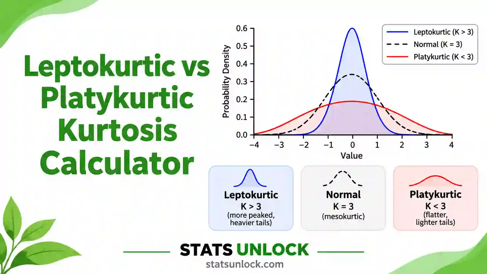

Leptokurtic vs Platykurtic Kurtosis Calculator
Paste comma-separated numbers or upload a CSV and find out in one click whether each group is leptokurtic, platykurtic or mesokurtic. You get excess kurtosis in all three software conventions, the standard error of kurtosis, a z test, the Anscombe-Glynn test, a bootstrap confidence interval and four colourful plots that show exactly which values drive the tails.
⚡ 0. Quick Answer
Leptokurtic vs platykurtic describes the tails of a distribution: a leptokurtic distribution has heavy tails and positive excess kurtosis (above 0), a platykurtic distribution has light tails and negative excess kurtosis (below 0), and a normal, mesokurtic distribution has excess kurtosis of exactly 0.
Kurtosis is the average of the fourth power of the z-scores. Because each z-score is raised to the fourth power, a few extreme values decide almost the whole number. Kurtosis is a measure of tails and outliers, not a measure of how pointed the peak looks.
Rule of thumb: excess kurtosis above +0.5 is leptokurtic, below −0.5 is platykurtic, and between the two is close to mesokurtic. For a normality check, an absolute value up to 2 is usually acceptable, and a z value (kurtosis ÷ SE) beyond ±1.96 is significant at the 5% level.
Key takeaways
- Leptokurtic vs platykurtic is a question about the tails: excess kurtosis > 0 means heavier tails than the normal curve, < 0 means lighter tails.
- The normal distribution has a Pearson kurtosis of 3 and an excess kurtosis of 0, so always check which one your software prints.
- Excel
KURT, SPSS and SAS report the bias-corrected G₂, while SciPy and the R moments package report the raw g₂; for n = 20 they can differ by more than 1.2. - Divide kurtosis by its standard error: |z| > 1.96 is significant at 5%, and for samples of 50 to 300 the usual normality cut-off is |z| < 3.29.
- In the worked example, just 2 of 20 scores produce 88.9% of the kurtosis, which is why you must look at the tails, not the peak.
📚 1. What Is Leptokurtic vs Platykurtic?
Kurtosis is a number that describes the shape of a distribution's tails. It answers one question: compared with a normal curve that has the same mean and standard deviation, does this data set produce more extreme values or fewer? The three names come from Greek words. Lepto means slender, platy means broad and flat, and meso means middle.
- Leptokurtic (excess kurtosis > 0): heavy tails. Extreme values happen more often than the normal curve predicts. Stock returns, insurance claims and animal movement distances are classic examples. The Laplace distribution has excess kurtosis of +3, and Student's t with 5 degrees of freedom has +6.
- Mesokurtic (excess kurtosis ≈ 0): normal tails. The normal distribution is the reference, with excess kurtosis of exactly 0.
- Platykurtic (excess kurtosis < 0): light tails. Values are spread evenly with few extremes, often because a scale has hard limits. A uniform distribution has excess kurtosis of −1.2, and the lowest possible value is −2, reached by a coin toss coded 0 and 1.
What it actually measures: kurtosis is the average of the z-scores raised to the fourth power. A value 1 SD from the mean adds 1 to that average, but a value 3 SD away adds 81. So the number is driven almost entirely by the tails. The old textbook story that kurtosis measures "peakedness" is not correct, and Westfall (2014) shows that two distributions with the same peak can have very different kurtosis.
A worked one-liner: for Class A in the default data (n = 20, mean 51.25), the fourth central moment is 4395.09 and the variance (m₂) is 27.69, so Pearson kurtosis = 4395.09 ÷ 27.69² = 5.733 and excess kurtosis g₂ = 5.733 − 3 = 2.733. The bias-corrected value that Excel prints is G₂ = 3.936. Both say: leptokurtic.
Who uses it: psychologists and social scientists check kurtosis before running t-tests, ANOVA or structural equation models. Finance teams use it to judge "fat tail" risk. Ecologists see leptokurtic dispersal kernels, where most seeds or animals move a short distance and a few travel very far. Quality engineers watch for platykurtic output, which can mean two machines are mixed in one batch.
| Feature | Leptokurtic | Mesokurtic | Platykurtic |
|---|---|---|---|
| Excess kurtosis | Greater than 0 | About 0 | Less than 0 (minimum −2) |
| Pearson kurtosis | Greater than 3 | About 3 | Less than 3 (minimum 1) |
| Tails | Heavy, more outliers | Normal | Light, few outliers |
| Q-Q plot shape | S-shape, ends bend away | Straight line | Inverted S, ends bend in |
| Typical example | Daily stock returns, Laplace, Student's t | Measurement error, heights in one group | Uniform, rating scales, two mixed groups |
| Risk for tests on means | Variance tests and CIs too optimistic | None | Usually mild, tests become slightly conservative |
Kurtosis vs skewness: skewness (the third moment) tells you whether one tail is longer than the other. Kurtosis (the fourth moment) tells you how heavy both tails are together. A distribution can be perfectly symmetric (skewness 0) and still be strongly leptokurtic, as the Laplace and t distributions are.
🧮 2. Set Up Your Data
Enter comma-separated numbers in each box (the default). Spaces, tabs, semicolons and new lines also work, so a column pasted from Excel is fine. Click a group name to rename it.
Type one value per cell. Each column becomes a group, and the header cell is its editable name. Empty cells are ignored.
📊 3. Results
How the number was calculated
Full results table
Normality and assumption checks
Which values drive the kurtosis?
Each value's share of Σz⁴. Kurtosis is a tail statistic, so a handful of extreme values usually supply most of it.
Visualisations
Four plots: the histogram against a normal curve, a normal Q-Q plot, excess kurtosis for every group with its confidence interval, and the tail shares compared with a normal distribution.
1. Histogram vs Normal Curve
Bars are your data, the line is a normal curve with the same mean and SD
2. Normal Q-Q Plot
S-shape means leptokurtic, inverted S means platykurtic
3. Excess Kurtosis by Group
Bars with confidence interval; dashed lines mark 0 and the ±2 normality limits
4. Tail Shares vs Normal
Share of values near the centre and beyond 1, 2 and 3 SD
🧠 4. Interpretation of Results, In Detail
4.1 What your kurtosis value actually tells you
Kurtosis compares the tails of your data with the tails of a normal curve that has the same mean and the same standard deviation. A positive excess kurtosis means your data produce extreme values more often than that normal curve would. A negative value means they produce fewer. That is the whole meaning of leptokurtic vs platykurtic, and nothing more.
Read the sign first, then the size. A value of +0.3 is a small departure that you can usually ignore. A value of +4 is a strong signal that a few values sit far from the rest. A value of −1.2 is what a perfectly flat, uniform spread of values gives, and values close to −2 almost always mean the data cluster at two ends, such as two separate groups mixed together.
4.2 Why kurtosis is about tails, not the peak
Many textbooks say a leptokurtic curve is "tall and thin" and a platykurtic curve is "flat-topped". This is the most common mistake about kurtosis. Because kurtosis averages z⁴, values within one standard deviation of the mean contribute at most 1 each to the total, while a single value 3 SD away contributes 81. Westfall (2014) proved that the central part of the data can only add a tiny, bounded amount to kurtosis.
The table Which values drive the kurtosis? in Section 3 shows this on your own data. In the default Class A data, the scores 66 and 38 together supply 88.9% of Σz⁴. Delete those two values and Class A becomes close to mesokurtic. So when you report a leptokurtic result, you are really reporting that your data contain a few extreme values.
4.3 Which kurtosis number did your software give you?
There are three formulas in common use, and they give different numbers on the same data. G₂ is the bias-corrected estimator printed by Excel's KURT, SPSS, SAS and pandas. g₂ is the plain moment estimator printed by SciPy's default and by R's moments package after you subtract 3. b₂ (Type 3) is printed by Minitab and by R's e1071 package by default. Joanes and Gill (1998) compared all three.
For large samples they agree. For small samples they do not: with n = 20 in Class A, G₂ = 3.94, g₂ = 2.73 and b₂ = 2.17. Always name the formula in your Methods section. And check whether a program prints excess kurtosis (normal = 0) or Pearson kurtosis (normal = 3), because a Pearson value of 2.8 is slightly platykurtic, not leptokurtic.
4.4 Is the result statistically significant?
A sample can show non-zero kurtosis just by chance, especially when it is small. Two tests answer whether the departure from 0 is real. The z ratio divides G₂ by its standard error and compares the result with ±1.96. It is simple and it is what SPSS users report, but it is too generous for small samples because the sampling distribution of kurtosis is strongly skewed. The Anscombe-Glynn test transforms the kurtosis first so the z value really follows a normal distribution, and it is what SciPy and R use.
In the default data, Class A has a z ratio of 3.97 but an Anscombe-Glynn z of only 2.52 (p = .012). Both say significant, but the gap shows how much the simple ratio can overstate the evidence. Class B is platykurtic by its value (−1.14) but not significant (p = .118), because 20 values are too few to tell a uniform spread from a normal one with confidence.
4.5 How large a value is a problem?
There is no single cut-off, and the right rule depends on sample size. For a quick normality screen, many methods texts accept an absolute excess kurtosis of up to 2. Kim (2013) gives a sample-size rule: for n under 50 use |z| < 1.96, for n from 50 to 300 use |z| < 3.29, and above 300 ignore z (it becomes significant for trivial departures) and look at the value itself, with an absolute kurtosis up to 7 still acceptable. The same limit of 7 is widely used before structural equation modelling. The checks table in Section 3 applies these rules for you.
4.6 What a leptokurtic result means for your analysis
Heavy tails matter more than light tails. Tests about means, such as the t-test and ANOVA, are fairly robust to kurtosis when groups are similar in size. But tests and intervals about variances are not. The F-test for equal variances, Bartlett's test and confidence intervals for a standard deviation can be badly wrong under leptokurtosis (Box, 1953). In structural equation modelling, positive kurtosis inflates the chi-square fit statistic and shrinks standard errors (Curran, West and Finch, 1996).
Good responses are: check the extreme values for errors, use robust methods such as trimmed means or Yuen's test, use Levene's or the Brown-Forsythe test instead of an F-test for variances, or bootstrap your confidence intervals.
4.7 What a platykurtic result means for your analysis
Light tails are usually harmless for tests on means; they make them slightly conservative. The bigger message is about where the data came from. Strong platykurtosis often means a bounded scale (a 1 to 7 rating scale used evenly), a floor or ceiling effect, or two subgroups mixed together. A value near −2 with a histogram that shows two humps is almost always a mixture. Darlington (1970) showed that negative kurtosis is closely linked to bimodality, so plot the data and look for a grouping variable you forgot to separate.
4.8 Kurtosis and skewness together
Always read kurtosis beside skewness. Skewness shows whether one tail is longer than the other; kurtosis shows how heavy the tails are overall. A long right tail (positive skew) usually also produces positive kurtosis, as in the sloth bear movement sample. The D'Agostino-Pearson K² test and the Jarque-Bera test combine both into one normality test. The calculator reports both, so you can see whether the shape problem is mainly asymmetry, mainly tail weight, or both.
4.9 Sample size changes everything
Kurtosis is the least stable of the common descriptive statistics. Its standard error is about √(24 ÷ n), so with n = 20 it is close to 1 and with n = 100 it is still about 0.48. Small samples often hide heavy tails completely, because the rare extreme values simply have not been drawn yet. Large samples flag tiny departures as significant. Report the value, the standard error and the confidence interval, and do not rely on the p-value alone.
4.10 Practical judgement
Use the shape label to describe your data, use the standard error and confidence interval to judge how sure you are, and use the driver table to find out which values are responsible. If one or two values supply most of Σz⁴, go back to the raw records before doing anything else. If the data are genuinely heavy-tailed, choose methods built for that. If they are platykurtic, check for a mixture or a bounded scale. Then write the result in plain words, as the templates in Section 5 show.
✍ 5. How to Write Your Results in Research
When reporting leptokurtic vs platykurtic results in APA format, give the kurtosis value, name the formula, add the standard error, and state the shape in words. Kurtosis is usually reported in the descriptive statistics part of the Results, next to the mean, SD and skewness.
▶ Run the analysis above to auto-fill all five examples with your results.
5.1 APA 7th edition results sentence
📌 Key conventions for this style
- Write p, z and SE in italics, and drop the leading zero for p (p = .012).
- Say "excess kurtosis" so no one confuses it with Pearson kurtosis, where normal = 3.
- Report two decimals for kurtosis and its SE, and exact p values down to p < .001.
- Put skewness and kurtosis in the same descriptive table as M and SD.
5.2 Thesis or dissertation Methods and Results
📌 Key conventions for this style
- Name the estimator (G₂, g₂ or b₂) and cite Joanes and Gill (1998).
- State the decision rule you used for normality and cite it, such as Kim (2013).
- Explain what you did about extreme values and whether the conclusion changed without them.
- Name the software and version.
5.3 Plain-language summary
📌 Key conventions for this style
- Say "more extreme values than expected" instead of "leptokurtic".
- Never say "peaked" or "flat-topped"; describe the tails.
- Give one concrete example, such as which values were far from the rest.
- Avoid symbols, p-values and Greek letters.
5.4 Structured abstract or conference poster
📌 Key conventions for this style
- Keep it to one line per group.
- Use the shape word in the headline: "Returns were strongly leptokurtic".
- Put the Q-Q plot on the poster; it shows kurtosis faster than any number.
- Footnote the estimator once.
5.5 Replication or pre-registration statement
📌 Key conventions for this style
- Fix the estimator, the test, the alpha and the cut-off before you see the data.
- Say in advance what you will do if kurtosis exceeds the limit (robust test, transformation, bootstrap).
- State the bootstrap seed and number of resamples so others get the same interval.
- Report the outlier rule and whether it is applied before or after the kurtosis check.
5.6 Table and figure conventions
In a descriptive statistics table, add two columns after M and SD: Skewness (SE) and Kurtosis (SE), for example 3.94 (0.99). Add a note under the table: "Kurtosis is excess kurtosis (G₂); the normal distribution has a value of 0." For a figure, a normal Q-Q plot is the clearest picture of kurtosis. Plot 2 in Section 3 is ready to use.
5.7 The Discussion sentence
Link the shape to its consequence: "Because scores were leptokurtic, variance-based tests were replaced with Levene's test, and confidence intervals were bootstrapped." Reviewers want to know what you did about the shape, not only that you measured it.
5.8 Reporting checklist
- The kurtosis value, with the formula named (G₂, g₂ or b₂) and "excess" stated.
- The standard error, and n for each group.
- The test used (z ratio or Anscombe-Glynn), the z value and the p value.
- The shape word, leptokurtic, platykurtic or mesokurtic, and the rule you used for it.
- Skewness next to kurtosis, and what you did if the data failed your normality rule.
∑ 6. Formulas Used
🔀 7. Kurtosis Calculation Flowchart, Step by Step
This flowchart shows how kurtosis is calculated, step by step, from a raw column of numbers to a leptokurtic, platykurtic or mesokurtic verdict. Every box uses the same worked example as the Excel, R and Python sections: the 20 exam scores of Class A.
Check any box yourself: the Excel sheet in Section 9, the R script in Section 10 and the Python script in Section 11 all return G₂ = 3.9365, g₂ = 2.7332 and SEK = 0.9924 for Class A, and G₂ = −1.1397 for Class B.
📝 8. How to Use This Calculator
- How to use this leptokurtic vs platykurtic calculator: enter your data. The default tab takes comma-separated numbers, exactly as the placeholder shows:
52, 48, 55, 61, 47, .... New lines, tabs, semicolons and spaces also work. - Name each group. The name field above every box is editable. Type something meaningful, such as Class A, morning, and it appears in the tables, charts and downloads.
- Add or remove groups. Press Add group to compare the shape of several samples side by side. Each group has its own Clear and Remove buttons.
- Or upload a file. On the Upload tab, choose a CSV or Excel file and click the column names you want. Every column you click becomes its own group, named after its header.
- Or type into the manual table and press Use this table to send it to the calculator.
- Try a sample dataset. Ten built-in data sets cover clear leptokurtic data (stock returns, bear movements), clear platykurtic data (uniform waiting times, mixed heights), a near-normal set, and a data-entry error that shows how one wrong value explodes kurtosis.
- Choose the kurtosis formula. Keep G₂ to match Excel and SPSS, or switch to g₂ or b₂ to match SciPy, R moments or Minitab.
- Set the shape band, the test, alpha and the bootstrap. The default ±0.5 band, the Anscombe-Glynn test, alpha = 0.05 and 2,000 seeded resamples suit most work.
- Press Run Kurtosis Analysis. Nothing is computed before you do, and changing any input clears the old results so you never read stale numbers.
- Read the verdict, check the plots and export. Start with the shape label and the driver table, look at the Q-Q plot, then copy a sentence from Section 5 or download the report as a text file or PDF.
📈 9. How to Calculate Kurtosis in Excel
Excel has one direct function for kurtosis, KURT, and it returns the bias-corrected excess kurtosis G₂, the same number SPSS prints. That part is easy. What trips people up is everything around it: Excel gives no standard error, no p-value and no shape label, and it has no function at all for the moment version g₂ that SciPy and many papers use. This section builds all of them, with the spreadsheet shown at each stage, using the Class A and Class B scores.
=KURT(A2:A21) and press Enter. Class A returns 3.9365, so it is leptokurtic. Class B in B2:B21 returns −1.1397, so it is platykurtic.9.1 The functions you need
| You want | Excel function | Note |
|---|---|---|
| Excess kurtosis G₂ | =KURT(A2:A21) | Bias-corrected, needs at least 4 numbers, normal = 0 |
| Skewness G₁ | =SKEW(A2:A21) | Always report it next to kurtosis |
| Sample size n | =COUNT(A2:A21) | Use COUNT, not COUNTA, which also counts text |
| Mean | =AVERAGE(A2:A21) | Needed for the moment version |
| Fourth-power deviations | =SUMPRODUCT((A2:A21-C3)^4) | C3 holds the mean |
| Moment kurtosis g₂ | =SUMPRODUCT((A2:A21-C3)^4)/C2/VAR.P(A2:A21)^2-3 | Matches SciPy's default; VAR.P divides by n |
| p-value from z | =2*(1-NORM.S.DIST(ABS(C7),TRUE)) | Two-tailed |
| Analysis ToolPak | Data → Data Analysis → Descriptive Statistics | Prints the same KURT value; enable the ToolPak first in File → Options → Add-ins |
9.2 Step by step
1 Put each group in its own column
Type a label in row 1 and the values below it, one group per column. KURT ignores the text header, so the range can start at row 2.
Class A sits in A2:A21 and Class B in B2:B21. Only the first eight rows are shown.
2 Get n, the mean, skewness and kurtosis
Build a small summary block next to the data: the statistic name in column B and the value in column C.
=COUNT(A2:A21)=AVERAGE(A2:A21)=SKEW(A2:A21)=KURT(A2:A21)C5 holds =KURT(A2:A21) and returns 3.9365, the bias-corrected excess kurtosis G₂. Skewness in C4 is 0.6413.
3 Add the standard error and the z ratio
Excel has no function for the standard error of kurtosis, so type the formula once. It refers to n in C2.
=2*SQRT(6*C2*(C2-1)/((C2-2)*(C2+1)*(C2+3)))*SQRT((C2^2-1)/((C2-3)*(C2+5)))=C5/C6=2*(1-NORM.S.DIST(ABS(C7),TRUE))SE of kurtosis in C6 is 0.9924, z in C7 is 3.9667, and the two-tailed p in C8 is 0.00007.
4 Add the moment version and a shape label
The moment estimator g₂ lets you match SciPy and many textbooks, and an IF formula turns the number into a word.
=SUMPRODUCT((A2:A21-C3)^4)/C2/VAR.P(A2:A21)^2-3=IF(C5>0.5,"Leptokurtic",IF(C5<-0.5,"Platykurtic","Mesokurtic"))g₂ in C9 is 2.7332, and C10 labels Class A as Leptokurtic. Copy C2:C10 one column right and point it at B2:B21 to get Class B.
9.3 The awkward cases
The p-value. Excel only gives you the simple z ratio. The Anscombe-Glynn test that SciPy and R use needs a longer formula. For Class A, Excel's z ratio of 3.97 gives p = .00007, while the Anscombe-Glynn test gives z = 2.52 and p = .012. Both are "significant", but the Excel version overstates the evidence for small samples.
=2*(1-NORM.S.DIST(ABS(KURT(A2:A21)/C6),TRUE))
Pearson kurtosis (normal = 3). If a paper or Stata reports kurtosis around 3, compare it with g₂ + 3, not with KURT.
=SUMPRODUCT((A2:A21-C3)^4)/C2/VAR.P(A2:A21)^2
For Class A this returns 5.7332. That is 2.7332 + 3, not a different result.
Fewer than four values. KURT returns #DIV/0! when there are fewer than four numbers or when every value is the same, because the variance is zero.
9.4 Why your Excel answer might differ from R, Python or SPSS
| Situation | What happens | Fix |
|---|---|---|
| SciPy gives 2.7332, Excel gives 3.9365 | scipy.stats.kurtosis defaults to bias=True, the moment estimator g₂ | Use bias=False to match KURT |
R moments::kurtosis gives 5.7332 | It returns Pearson kurtosis (normal = 3), not excess | Subtract 3, then you have g₂ |
R e1071::kurtosis gives 2.1743 | Its default is type 3 (b₂) | Use type = 2 to match Excel |
Stata summarize, detail gives 5.733 | Stata prints Pearson kurtosis with the moment formula | Subtract 3, then compare with g₂ |
| Excel p-value is far smaller than R's | Excel route uses z = G₂ ÷ SE; R and SciPy use Anscombe-Glynn | Name the test you used; prefer Anscombe-Glynn for n under 100 |
| Blank or text cells | KURT skips them, so n is smaller than you think | Check COUNT first |
| Zeros used for missing data | Zeros are real values and can create fake heavy tails | Delete them or use a blank |
SciPy's normaltest looks odd when skewness is exactly 0 | SciPy's skewness test replaces an exact zero with 1 internally, so its K² is slightly too large | This page treats zero skewness as z = 0; the kurtosis part is identical |
| Bootstrap intervals differ slightly | Each program uses a different random number generator | Expected; the page uses seed 42 and 2,000 resamples |
| Software | Command | What it prints | Class A value |
|---|---|---|---|
| Excel / Google Sheets | =KURT(rng) | G₂, excess | 3.9365 |
| SPSS, SAS, pandas | Descriptives / PROC MEANS / df.kurt() | G₂, excess | 3.9365 |
| SciPy default | stats.kurtosis(x) | g₂, excess | 2.7332 |
| R moments | moments::kurtosis(x) | Pearson, normal = 3 | 5.7332 |
| R e1071, Minitab | e1071::kurtosis(x) | b₂, excess | 2.1743 |
| Stata | summarize x, detail | Pearson, normal = 3 | 5.7332 |
9.5 Charting kurtosis in Excel
- Select the data column and choose Insert → Charts → Histogram (Excel 2016 or later).
- Right-click the horizontal axis, choose Format Axis, and set a sensible bin width so you can see the tails.
- For a Q-Q plot, sort the data in a new column, add
=NORM.S.INV((ROW()-1-0.375)/(COUNT(A:A)+0.25))beside it, standardise the data with=STANDARDIZE(x, mean, sd), and draw an XY scatter of the two columns. - Add a straight line through the origin with slope 1. Points that curve away at both ends show leptokurtosis; points that bend inward show platykurtosis.
Plots 1 and 2 in Section 3 draw the histogram with a normal curve and the Q-Q plot automatically, which is much faster than building them in Excel.
9.6 Excel errors you will probably hit
| Excel shows | Why | Fix |
|---|---|---|
#DIV/0! from KURT | Fewer than 4 numbers, or all values identical | Add data; a constant column has no kurtosis |
#VALUE! | Text or a unit typed into a cell used by SUMPRODUCT | Keep units in the header only |
#NUM! in the SE formula | n is below 4, so a square root of a negative number appears | Check that C2 holds the right count |
#NAME? | Typed KURTOSIS or NORMSDIST in a new version | Use KURT and NORM.S.DIST |
| Kurtosis is huge, such as 19.88 | One typing error, such as 520 for 52 | Sort the column and look at both ends |
| Green triangles in cells | Numbers stored as text and silently skipped | Select, click the warning icon, Convert to Number |
📈 10. How to Calculate Kurtosis in R
R has no built-in kurtosis function in base R, and the two popular packages disagree with each other and with Excel. The script below avoids that confusion. It uses base R only, computes all three kurtosis conventions, the standard error, the z ratio and the Anscombe-Glynn test, prints a plain-English verdict for every group, and saves one publication-ready figure at 300 dpi.
Rscript. Change only the groups <- list(...) lines to use your own data.10.1 The complete script
R, base only, saves kurtosis_plot.png
# ============================================================
# Leptokurtic vs platykurtic: kurtosis, SE, tests and one plot
# StatsUnlock - https://statsunlock.com/leptokurtic-vs-platykurtic-kurtosis-calculator/
# Base R only. No packages to install.
# ============================================================

# ---- 1. Your data ------------------------------------------
# Replace with your own values, or read a CSV:
#   d <- read.csv("data.csv")
#   groups <- list("Class A" = d$score[!is.na(d$score)])
groups <- list(
  "Class A" = c(52, 48, 55, 61, 47, 50, 51, 49, 53, 50,
                52, 51, 50, 49, 52, 50, 51, 38, 66, 50),
  "Class B" = c(41, 44, 46, 48, 50, 52, 54, 56, 58, 60,
                62, 43, 47, 51, 55, 59, 63, 45, 49, 57)
)

# ---- 2. Kurtosis in all three conventions ------------------
kurt_all <- function(x) {
  x  <- x[!is.na(x)]                      # drop missing values
  n  <- length(x)
  d  <- x - mean(x)
  m2 <- mean(d^2); m3 <- mean(d^3); m4 <- mean(d^4)
  g2 <- m4 / m2^2 - 3                                       # moments, SciPy default
  G2 <- ((n + 1) * g2 + 6) * (n - 1) / ((n - 2) * (n - 3))  # Excel KURT, SPSS
  b2 <- (g2 + 3) * (1 - 1 / n)^2 - 3                        # type 3, e1071 default
  G1 <- m3 / m2^1.5 * sqrt(n * (n - 1)) / (n - 2)           # skewness, Excel SKEW
  ses <- sqrt(6 * n * (n - 1) / ((n - 2) * (n + 1) * (n + 3)))
  sek <- 2 * ses * sqrt((n^2 - 1) / ((n - 3) * (n + 5)))
  # Anscombe-Glynn test, same as moments::anscombe.test and scipy kurtosistest
  b    <- m4 / m2^2
  E    <- 3 * (n - 1) / (n + 1)
  varb <- 24 * n * (n - 2) * (n - 3) / ((n + 1)^2 * (n + 3) * (n + 5))
  xs   <- (b - E) / sqrt(varb)
  sb1  <- 6 * (n^2 - 5 * n + 2) / ((n + 7) * (n + 9)) *
          sqrt(6 * (n + 3) * (n + 5) / (n * (n - 2) * (n - 3)))
  A    <- 6 + 8 / sb1 * (2 / sb1 + sqrt(1 + 4 / sb1^2))
  den  <- 1 + xs * sqrt(2 / (A - 4))
  t2   <- sign(den) * ((1 - 2 / A) / abs(den))^(1 / 3)
  z_ag <- (1 - 2 / (9 * A) - t2) / sqrt(2 / (9 * A))
  list(n = n, g2 = g2, G2 = G2, b2 = b2, G1 = G1, sek = sek,
       z = G2 / sek, z_ag = z_ag, p_ag = 2 * pnorm(-abs(z_ag)))
}

shape <- function(k, band = 0.5) {
  if (k > band) "leptokurtic (heavy tails)"
  else if (k < -band) "platykurtic (light tails)"
  else "mesokurtic (close to normal)"
}

# ---- 3. Print the results ----------------------------------
res <- lapply(groups, kurt_all)
for (g in names(res)) {
  r <- res[[g]]
  cat(sprintf("\n%s (n = %d)\n", g, r$n))
  cat(sprintf("  Excess kurtosis G2 = %.4f   g2 = %.4f   b2 = %.4f\n", r$G2, r$g2, r$b2))
  cat(sprintf("  SE of kurtosis     = %.4f   z = G2/SE = %.4f\n", r$sek, r$z))
  cat(sprintf("  Anscombe-Glynn z   = %.4f   p = %.4f\n", r$z_ag, r$p_ag))
  cat(sprintf("  Skewness G1        = %.4f\n", r$G1))
  cat(sprintf("  Verdict: %s, %s at alpha = 0.05\n", shape(r$G2),
      if (r$p_ag < 0.05) "significantly different from normal"
      else "not significantly different from normal"))
}

# ---- 4. Seeded bootstrap 95% CI for G2 ---------------------
set.seed(42)
for (g in names(groups)) {
  bs <- replicate(2000, kurt_all(sample(groups[[g]], replace = TRUE))$G2)
  ci <- quantile(bs, c(0.025, 0.975), na.rm = TRUE)
  cat(sprintf("Bootstrap 95%% CI for G2, %s: %.2f to %.2f\n", g, ci[1], ci[2]))
}

# ---- 5. One figure: histogram + normal curve per group -----
png("kurtosis_plot.png", width = 1200 * length(groups), height = 1100, res = 300)
par(mfrow = c(1, length(groups)), mar = c(4.2, 4.2, 3, 1))
for (g in names(groups)) {
  x <- groups[[g]]; r <- res[[g]]
  col <- if (r$G2 > 0.5) "#9333ea" else if (r$G2 < -0.5) "#0d9488" else "#16a34a"
  h <- hist(x, breaks = "Sturges", plot = FALSE)
  xs <- seq(min(x) - sd(x), max(x) + sd(x), length.out = 200)
  ys <- dnorm(xs, mean(x), sd(x))
  plot(h, freq = FALSE, col = adjustcolor(col, 0.55), border = "white",
       ylim = c(0, max(h$density, ys) * 1.1), xlim = range(xs),
       main = sprintf("%s: G2 = %.2f", g, r$G2), xlab = "Value", cex.main = 0.95)
  lines(xs, ys, col = "#2563eb", lwd = 2)
  mtext(shape(r$G2), side = 3, line = 0.2, cex = 0.7)
}
invisible(dev.off())
cat("\nSaved kurtosis_plot.png\n")
Run it with Rscript kurtosis.R from a terminal, or paste it into the RStudio console. Class A prints G2 = 3.9365, g2 = 2.7332, SE = 0.9924 and Anscombe-Glynn p = 0.0118. Class B prints G2 = −1.1397 and p = 0.1182. The bootstrap interval differs a little from this page because R uses a different random generator.
10.2 What each part does
| Line or function | What it does, and why it is there |
|---|---|
| groups <- list(...) | One named vector per group. The names become the labels in the printout and the figure. |
| x[!is.na(x)] | Drops missing values. Without it, mean() returns NA and every result becomes NA. |
| mean(d^4) | The fourth central moment m₄, with n in the denominator. This is the heart of kurtosis. |
| g2, G2, b2 | The three conventions. G2 matches Excel and SPSS, g2 matches SciPy, b2 matches e1071 and Minitab. |
| sek | The standard error of kurtosis printed by SPSS. Divide G2 by it to get the z ratio. |
| A, den, t2, z_ag | The Anscombe-Glynn transformation. It turns the skewed sampling distribution of kurtosis into a z value that really is close to normal. |
| pnorm(-abs(z_ag)) | The one-sided tail area; doubling it gives the two-tailed p-value. |
| set.seed(42) | Fixes the bootstrap so you get the same interval every run. |
| replicate(2000, ...) | Resamples the data 2,000 times with replacement and recomputes G2 each time. |
| png(..., res = 300) | Writes a 300 dpi file. Without res you get a blurry 72 dpi image. |
| dnorm(xs, mean, sd) | The normal curve with the same mean and SD, the reference for judging tails. |
| dev.off() | Closes the file. Forgetting it leaves an empty or locked PNG. |
10.3 What the figure shows
Two panels sit side by side. For Class A the purple bars pile up near 50 and two isolated bars sit far out at 38 and 66, beyond where the blue normal curve has almost no height: that is the leptokurtic signature. For Class B the teal bars are spread evenly and stop before the normal curve's tails do: that is the platykurtic signature.
10.4 Common R problems and fixes
| Problem | Cause | Fix |
|---|---|---|
| kurtosis() gives about 5.7 | moments package returns Pearson kurtosis | Subtract 3, or use this script |
| e1071 and SPSS disagree | e1071 default is type 3 | e1071::kurtosis(x, type = 2) |
| Error: could not find function "kurtosis" | Base R has none | Use kurt_all() above |
| All results are NA | Missing values in the vector | Keep the !is.na line |
| NaN for n = 3 | G2 divides by (n − 3) | Kurtosis needs n of at least 4 |
| Warning in quantile about NA | A bootstrap sample with all equal values | Harmless; na.rm = TRUE handles it |
| Plot file is empty | dev.off() not reached | Run the whole script, not part of it |
10.5 Useful one-liners
e1071::kurtosis(x, type = 2)                 # same as Excel KURT
moments::kurtosis(x) - 3                     # g2, the SciPy default
moments::anscombe.test(x)                    # Anscombe-Glynn test
sapply(split(d$y, d$group), function(v) kurt_all(v)$G2)   # per group
qqnorm(x); qqline(x)                         # quick Q-Q plot
write.csv(do.call(rbind, lapply(res, unlist)), "kurtosis.csv")
📈 11. How to Calculate Kurtosis in Python
Python's scipy.stats.kurtosis(x) is one line, but its default is the moment estimator g₂, not the bias-corrected G₂ that Excel and SPSS print. The script below sets it explicitly, adds the standard error, the z ratio, the Anscombe-Glynn test and a seeded bootstrap interval, prints a plain verdict for each group, and saves one 300 dpi figure.
groups = {...} lines.Install with pip install numpy scipy matplotlib. Add pandas only if you read a CSV.
11.1 The complete script
Python 3, saves kurtosis_plot.png
# ============================================================
# Leptokurtic vs platykurtic: kurtosis, SE, tests and one plot
# StatsUnlock - https://statsunlock.com/leptokurtic-vs-platykurtic-kurtosis-calculator/
# ============================================================
import numpy as np
from scipy import stats
import matplotlib.pyplot as plt

# ---- 1. Your data ------------------------------------------
# Or read a CSV:
#   import pandas as pd
#   df = pd.read_csv("data.csv")
#   groups = {"Class A": df["score"].dropna().to_numpy()}
groups = {
    "Class A": [52, 48, 55, 61, 47, 50, 51, 49, 53, 50,
                52, 51, 50, 49, 52, 50, 51, 38, 66, 50],
    "Class B": [41, 44, 46, 48, 50, 52, 54, 56, 58, 60,
                62, 43, 47, 51, 55, 59, 63, 45, 49, 57],
}

def shape(k, band=0.5):
    if k > band:
        return "leptokurtic (heavy tails)"
    if k < -band:
        return "platykurtic (light tails)"
    return "mesokurtic (close to normal)"

rng = np.random.default_rng(42)          # seeded bootstrap
fig, axes = plt.subplots(1, len(groups), figsize=(4.6 * len(groups), 4.0))
axes = np.atleast_1d(axes)

for ax, (name, values) in zip(axes, groups.items()):
    x = np.asarray(values, dtype=float)
    x = x[~np.isnan(x)]                   # drop missing values
    n = len(x)

    # ---- 2. Kurtosis in all three conventions ---------------
    G2 = stats.kurtosis(x, fisher=True, bias=False)   # Excel KURT, SPSS, pandas
    g2 = stats.kurtosis(x, fisher=True, bias=True)    # SciPy default
    b2 = (g2 + 3) * (1 - 1 / n) ** 2 - 3              # type 3, Minitab
    G1 = stats.skew(x, bias=False)                     # Excel SKEW

    ses = np.sqrt(6 * n * (n - 1) / ((n - 2) * (n + 1) * (n + 3)))
    sek = 2 * ses * np.sqrt((n ** 2 - 1) / ((n - 3) * (n + 5)))
    z_ag, p_ag = stats.kurtosistest(x)                # Anscombe-Glynn

    boot = [stats.kurtosis(rng.choice(x, n, replace=True), bias=False)
            for _ in range(2000)]
    lo, hi = np.nanpercentile(boot, [2.5, 97.5])

    # ---- 3. Print the results -------------------------------
    print(f"\n{name} (n = {n})")
    print(f"  Excess kurtosis G2 = {G2:.4f}   g2 = {g2:.4f}   b2 = {b2:.4f}")
    print(f"  SE of kurtosis     = {sek:.4f}   z = G2/SE = {G2 / sek:.4f}")
    print(f"  Anscombe-Glynn z   = {z_ag:.4f}   p = {p_ag:.4f}")
    print(f"  Skewness G1        = {G1:.4f}")
    print(f"  Bootstrap 95% CI for G2: {lo:.2f} to {hi:.2f}")
    verdict = "significantly" if p_ag < 0.05 else "not significantly"
    print(f"  Verdict: {shape(G2)}, {verdict} different from normal at alpha = 0.05")

    # ---- 4. Histogram with a matching normal curve ----------
    col = "#9333ea" if G2 > 0.5 else ("#0d9488" if G2 < -0.5 else "#16a34a")
    ax.hist(x, bins="sturges", density=True, color=col, alpha=0.6, edgecolor="white")
    xs = np.linspace(x.min() - x.std(ddof=1), x.max() + x.std(ddof=1), 200)
    ax.plot(xs, stats.norm.pdf(xs, x.mean(), x.std(ddof=1)), color="#2563eb", lw=2)
    ax.set_title(f"{name}: G2 = {G2:.2f}\n{shape(G2)}", fontsize=10)
    ax.set_xlabel("Value")
    ax.set_ylabel("Density")

fig.tight_layout()
fig.savefig("kurtosis_plot.png", dpi=300, bbox_inches="tight")
print("\nSaved kurtosis_plot.png")
11.2 What each part does
| Line or function | What it does, and why it is there |
|---|---|
| dtype=float | Makes sure integer data are not handled with integer arithmetic. |
| x[~np.isnan(x)] | Drops missing values. NumPy functions return nan if any value is nan. |
| bias=False | Gives G2, the Excel and SPSS value. The default bias=True gives g2, which is smaller for small samples. |
| fisher=True | Returns excess kurtosis (normal = 0). fisher=False returns Pearson kurtosis (normal = 3). |
| stats.kurtosistest | The Anscombe-Glynn test. It warns when n is below 20, because the test is less accurate there. |
| np.random.default_rng(42) | A seeded generator, so the bootstrap interval is the same every run. |
| np.nanpercentile | The percentile interval, ignoring the rare resample where every value is the same. |
| x.std(ddof=1) | The sample SD that matches Excel's STDEV.S. np.std alone divides by n. |
| fig.savefig(..., dpi=300) | Writes a print-quality file. bbox_inches="tight" trims empty margins. |
11.3 What the figure shows
The same two panels as the R figure: purple bars for Class A with isolated values at 38 and 66 sitting in the far tails of the blue normal curve, and teal bars for Class B that fill the middle evenly and stop short of the normal tails.
11.4 Common Python problems and fixes
| Problem | Cause | Fix |
|---|---|---|
| Kurtosis differs from Excel | SciPy default is bias=True | Pass bias=False |
| Value near 3 for normal data | fisher=False was used | Use fisher=True |
| Result is nan | Missing values in the array | Keep the isnan line or use nan_policy="omit" |
| UserWarning from kurtosistest | n is below 20 | Report the value and SE; treat the p-value with care |
| pandas and SciPy disagree | df.kurt() is G2, SciPy default is g2 | Match with bias=False |
| normaltest differs from this page | SciPy's skew test treats an exact zero skewness as 1 | Only affects perfectly symmetric data; the kurtosis test is identical |
| Figure window never appears | Script only saves the file | Add plt.show() in Jupyter |
11.5 Useful one-liners
stats.kurtosis(x, bias=False)                     # same as Excel KURT
stats.kurtosis(x, fisher=False)                   # Pearson kurtosis, normal = 3
stats.kurtosistest(x)                             # Anscombe-Glynn z and p
stats.normaltest(x)                               # D'Agostino-Pearson K2
stats.jarque_bera(x)                              # Jarque-Bera test
df.groupby("group")["y"].apply(lambda s: s.kurt())  # per group, pandas
stats.probplot(x, dist="norm", plot=plt)          # quick Q-Q plot
Run it with python kurtosis.py. Class A prints G2 = 3.9365, g2 = 2.7332, SE = 0.9924, z = 2.5173 and p = 0.0118, the same as R, Excel and this page.
📋 12. Reference Tables
12.1 Kurtosis of common distributions
| Distribution | Excess kurtosis | Pearson kurtosis | Shape |
|---|---|---|---|
| Two-point (coin toss, p = 0.5) | −2.000 | 1.000 | Platykurtic, the minimum |
| Uniform | −1.200 | 1.800 | Platykurtic |
| Beta(2, 2) | −0.857 | 2.143 | Platykurtic |
| Triangular (symmetric) | −0.600 | 2.400 | Platykurtic |
| Normal | 0.000 | 3.000 | Mesokurtic, the reference |
| Logistic | 1.200 | 4.200 | Leptokurtic |
| Student's t, 10 df | 1.000 | 4.000 | Leptokurtic |
| Laplace (double exponential) | 3.000 | 6.000 | Leptokurtic |
| Lognormal, σ = 0.5 | 5.898 | 8.898 | Leptokurtic and skewed |
| Exponential | 6.000 | 9.000 | Leptokurtic and skewed |
| Student's t, 5 df | 6.000 | 9.000 | Strongly leptokurtic |
| Student's t, 4 df or fewer | Undefined (infinite) | Undefined | Tails too heavy for a fourth moment |
What to conclude: a symmetric distribution can be either leptokurtic or platykurtic, and the theoretical floor is −2. Values follow from the standard moment formulas; see Balanda and MacGillivray (1988) and DeCarlo (1997).
12.2 Standard error of kurtosis and the critical value by sample size
| n | SE of skewness | SE of kurtosis | |G₂| needed for p < .05 (z ratio) | |G₂| needed for p < .01 |
|---|---|---|---|---|
| 10 | 0.687 | 1.334 | 2.62 | 3.44 |
| 15 | 0.580 | 1.121 | 2.20 | 2.89 |
| 20 | 0.512 | 0.992 | 1.95 | 2.56 |
| 30 | 0.427 | 0.833 | 1.63 | 2.15 |
| 50 | 0.337 | 0.662 | 1.30 | 1.71 |
| 100 | 0.241 | 0.478 | 0.94 | 1.23 |
| 200 | 0.172 | 0.342 | 0.67 | 0.88 |
| 300 | 0.141 | 0.281 | 0.55 | 0.72 |
| 500 | 0.109 | 0.218 | 0.43 | 0.56 |
| 1000 | 0.077 | 0.155 | 0.30 | 0.40 |
What to conclude: with 20 values you need |G₂| near 2 to call kurtosis significant, while with 1,000 values even 0.3 is significant. This is why Kim (2013) changes the rule with sample size.
12.3 How to describe the size of excess kurtosis
| |Excess kurtosis| | Description | Typical action |
|---|---|---|
| Below 0.5 | Close to mesokurtic | Treat tails as normal |
| 0.5 to 1.0 | Mild | Report it; most tests on means are fine |
| 1.0 to 2.0 | Moderate | Look at the Q-Q plot; avoid variance tests that assume normality |
| 2.0 to 7.0 | Substantial | Check extreme values; consider robust or bootstrap methods |
| Above 7.0 | Severe | Normal-theory methods are unsafe; transform, model the tails, or use robust estimators |
What to conclude: these are practical labels, not formal tests. The limits of 2 and 7 come from the normality rules used in Kim (2013) and the simulation design of Curran, West and Finch (1996).
12.4 Acceptable kurtosis range for normality, by rule
| Rule | Sample size | Accept normal tails when |
|---|---|---|
| z test at 5% | n < 50 | |G₂ ÷ SE| < 1.96 |
| Kim (2013) | 50 to 300 | |G₂ ÷ SE| < 3.29 |
| Kim (2013) | above 300 | |excess kurtosis| < 7 |
| Common screening rule | any | |excess kurtosis| ≤ 2 |
| Curran, West and Finch (1996) | SEM studies | Kurtosis near 7 is already "moderate" non-normality |
What to conclude: always state which rule you used. The checks table in Section 3 applies the z rule, Kim's rule and the ±2 rule at the same time.
12.5 Share of values in the centre and the tails
| Distribution | Within ±0.5 SD | Beyond ±1 SD | Beyond ±2 SD | Beyond ±3 SD |
|---|---|---|---|---|
| Uniform (platykurtic) | 28.87% | 42.26% | 0.00% | 0.00% |
| Normal (mesokurtic) | 38.29% | 31.73% | 4.55% | 0.27% |
| Logistic (leptokurtic) | 42.47% | 28.04% | 5.18% | 0.86% |
| Student's t, 5 df | 45.29% | 25.32% | 4.93% | 1.17% |
| Laplace (leptokurtic) | 50.69% | 24.31% | 5.91% | 1.44% |
What to conclude: heavy-tailed distributions have more values beyond 3 SD (about five times as many for the Laplace) and also more near the centre, with fewer in the "shoulders" between. Plot 4 in Section 3 compares your data with the normal row.
12.6 Moors' robust kurtosis
| Distribution | Moors kurtosis | Reading |
|---|---|---|
| Uniform | 1.000 | Lighter tails than normal |
| Normal | 1.233 | The reference value |
| Logistic | 1.306 | Heavier tails |
| Student's t, 5 df | 1.327 | Heavier tails |
| Laplace | 1.585 | Much heavier tails |
What to conclude: Moors (1988) uses octiles instead of fourth powers, so one wild value cannot dominate it. If the moment kurtosis is large but Moors is near 1.233, a few outliers are doing all the work.
📈 13. Example Results
Eight worked examples show leptokurtic vs platykurtic results across the situations you will meet. Every value uses G₂ (Excel KURT) and the Anscombe-Glynn test unless stated. Load the same data from the sample dropdown in Section 2 to reproduce them.
Exam scores in Class A
The default data: a tight middle with two far-out scores.
Twenty students sat the same exam. Most scored between 47 and 55, one scored 38 and one scored 66.
| Statistic | Value | Note |
|---|---|---|
| Mean (SD) | 51.25 (5.40) | Centre and spread |
| G₂ / g₂ / b₂ | 3.94 / 2.73 / 2.17 | Three conventions |
| z ratio | 3.97 | G₂ ÷ SE |
| Anscombe-Glynn z, p | 2.52, .012 | Significant |
| Skewness G₁ | 0.64 | Mild right skew |
| Share of Σz⁴ from 66 and 38 | 88.9% | Two values decide it |
What it means: Class A is leptokurtic. The heavy tails come from just two students, so the right next step is to confirm those two scores and to report the result with that in mind.
How to write it: "Scores in Class A were leptokurtic (G₂ = 3.94, SE = 0.99; Anscombe-Glynn z = 2.52, p = .012), driven by two extreme scores (38 and 66)."
Daily stock returns
Fat tails, the classic finance case.
Thirty daily returns in percent. Most days move less than half a percent, but three days move 1.8%, 3.6% and −4.1%.
| Statistic | Value | Note |
|---|---|---|
| Mean (SD) | 0.07 (1.09) | Percent per day |
| G₂ | 10.61 | Far above 2 and 7 |
| Anscombe-Glynn z, p | 4.10, < .001 | Highly significant |
| Skewness G₁ | −0.67 | The crash day is the biggest |
| Share from −4.1 alone | 64.8% | One day dominates |
What it means: A normal model would call a −4.1% day a near-impossible event. Heavy tails like this are why risk models use Student's t or other fat-tailed distributions (Cont, 2001).
How to write it: "Daily returns were strongly leptokurtic (G₂ = 10.61, SE = 0.83, p < .001), so a t distribution was used for value-at-risk."
Bus waiting times
The two tests disagree.
Twenty-four waiting times in minutes for a bus that comes every 12 minutes. Arrivals are random, so waits are spread evenly from 0 to 12.
| Statistic | Value | Note |
|---|---|---|
| Mean (SD) | 6.00 (3.54) | Minutes |
| G₂ | −1.27 | Near the uniform value −1.2 |
| z ratio, p | −1.38, .168 | Not significant |
| Anscombe-Glynn z, p | −2.16, .030 | Significant |
What it means: The simple z ratio misses this, because the sampling distribution of kurtosis is skewed and negative values are hard to reach in small samples. The Anscombe-Glynn test corrects for that and finds the light tails. Report the test you used.
How to write it: "Waiting times were platykurtic (G₂ = −1.27, SE = 0.92; Anscombe-Glynn z = −2.16, p = .030), consistent with a uniform distribution."
Machine part diameters
What mesokurtic looks like.
Thirty shaft diameters from one well-tuned machine, target 25.000 mm.
| Statistic | Value | Note |
|---|---|---|
| Mean (SD) | 25.000 (0.050) | mm |
| G₂ | −0.24 | Inside the ±0.5 band |
| Anscombe-Glynn z, p | −0.11, .911 | No evidence of non-normal tails |
| Skewness G₁ | 0.00 | Symmetric |
What it means: The tails match a normal curve. This does not prove the data are normal, only that there is no evidence against it in the tails.
How to write it: "Diameters were approximately mesokurtic (G₂ = −0.24, SE = 0.83, p = .911)."
Exam scores in Class B
Platykurtic by value, but not significant.
Twenty scores spread evenly from 41 to 63 with no clear centre.
| Statistic | Value | Note |
|---|---|---|
| Mean (SD) | 52.00 (6.61) | Score |
| G₂ / g₂ | −1.14 / −1.16 | Close to the uniform value |
| Anscombe-Glynn z, p | −1.56, .118 | Not significant |
| Moors kurtosis | 0.90 | Below the normal 1.233 |
What it means: The shape is clearly flat, but with 20 values a normal sample could look like this by chance. Describe it as platykurtic, and say that the test lacked power.
How to write it: "Class B scores were platykurtic (G₂ = −1.14, SE = 0.99), although the departure was not significant (z = −1.56, p = .118)."
Adult heights in a national survey
Large n makes tiny kurtosis significant.
Heights of 3,000 adults in centimetres, with very slightly heavier tails than normal.
| Statistic | Value | Note |
|---|---|---|
| Mean (SD) | 169.76 (6.76) | cm |
| G₂ | 0.27 | Inside the ±0.5 band |
| z ratio | 3.03 | Significant |
| Anscombe-Glynn z, p | 2.73, .006 | Significant |
| Kim (2013), n > 300 | |0.27| < 7 | Acceptable |
What it means: The test is significant because the sample is huge, not because the tails are a problem. Judge large samples by the size of the value, not by p.
How to write it: "Heights showed a negligible excess kurtosis (G₂ = 0.27, SE = 0.09); although significant (p = .006), the value is well within accepted limits for n = 3,000."
One typing error
520 typed instead of 52.
The Class A scores again, but one score of 52 was entered as 520.
| Statistic | Value | Note |
|---|---|---|
| Mean (SD) | 74.65 (104.96) | Both distorted |
| G₂ | 19.88 | Near the maximum for n = 20 |
| Anscombe-Glynn z, p | 4.69, < .001 | Meaningless here |
| Share of Σz⁴ from 520 | > 99.9% | One value is the whole result |
What it means: When one value supplies nearly all of Σz⁴, kurtosis is measuring that value, not the distribution. Correct it to 52 and G₂ falls back to 3.94.
How to write it: "One data-entry error (520 for 52) was identified from an extreme kurtosis value (G₂ = 19.88) and corrected before analysis."
Sloth bear daily travel distance
Most days short, a few very long.
Daily straight-line distances (km) for one radio-collared sloth bear over 25 days. Three days were long-range movements of 7.4, 9.8 and 12.6 km.
| Statistic | Value | Note |
|---|---|---|
| Mean (SD) | 3.59 (2.54) | km per day |
| Median | 2.80 | The typical day |
| G₂ | 7.24 | Severe |
| Anscombe-Glynn z, p | 3.46, < .001 | Significant |
| Share from 12.6 km | 79.2% | One long trip |
What it means: Animal movement and seed dispersal are typically leptokurtic: most moves are short and a few are very long (Kot, Lewis and van den Driessche, 1996). The long days are real behaviour, not errors, so model them with a heavy-tailed or log-scale distribution rather than deleting them.
How to write it: "Daily travel distance was right-skewed and leptokurtic (G₁ = 2.75, G₂ = 7.24, SE = 0.90; p < .001); the median of 2.8 km is reported as the typical daily distance."
🧪 14. Data Collection Protocol
Study design: kurtosis assumes a set of independent measurements of one numeric variable on an interval or ratio scale, collected from one well-defined population per group.
- Decide before collecting why you need kurtosis. Is it a normality check before another test, a description of risk in the tails, or the main outcome? The answer sets your sample size and your cut-off rule.
- Plan enough values for a leptokurtic vs platykurtic decision. Kurtosis needs at least 4 values to compute and about 20 for the Anscombe-Glynn test. For a confident shape verdict, aim for 50 or more per group, because rare tail values may not appear in small samples.
- Define one group per column. Mixing two populations, such as two age groups or two sites, creates artificial platykurtosis. Record the grouping variable so you can split the data later.
- Sample at random or systematically. Selecting "typical" cases removes the tails you are trying to measure and pushes kurtosis down.
- Fix the instrument and its range. A scale with a ceiling (such as a 1 to 7 rating) or a detection limit cuts off the tails and produces platykurtosis that is not real.
- Record values at full precision. Heavy rounding creates many tied values and can distort a kurtosis calculation in small samples.
- Never use 0 or 999 for missing data. A code like 999 becomes an extreme value and can push kurtosis close to its maximum on its own. Leave the cell blank.
- Double-enter or verify the extreme values. Because kurtosis is driven by the tails, check every value beyond 3 SD against the original record.
- Write the outlier rule in advance. Decide how real extreme values will be handled before you see the kurtosis, so the decision cannot be tuned to the result.
- Keep the time order if there is one. Kurtosis assumes independent values. If you measure the same subject repeatedly, note it, because correlated values make the standard error too small.
| Row | Class A | Class B | Notes |
|---|---|---|---|
| 1 | 52 | 41 | One student per row, one group per column |
| 2 | 48 | 44 | Blank cells allowed if group sizes differ |
| 3 | 55 | 46 | Numbers only; units go in the header |
Minimum sample: 4 to compute, 20 for the Anscombe-Glynn test, 50 or more per group for a reliable verdict, and a few hundred to estimate the size of heavy-tailed kurtosis with any precision. Pre-registration line: "Excess kurtosis (G₂) will be computed per group and judged with the Anscombe-Glynn test at α = .05 and Kim's (2013) rule." Common mistakes: pooling groups, using codes for missing data, and deleting extreme values before calculating kurtosis.
🎯 15. When to Use This Calculator
This free leptokurtic vs platykurtic calculator is designed for anyone who needs to describe the tails of a numeric variable or check them before choosing a statistical method.
Use it when:
- You must report skewness and kurtosis in a descriptive statistics table.
- You are checking normality before a t-test, ANOVA, regression or structural equation model.
- You want to know whether extreme values are more common than a normal model predicts, as in finance, insurance, hydrology or animal movement.
- You need to compare the tail shape of several groups side by side.
- You suspect a data-entry error or a mixture of two populations.
Do not use it when:
- Your data are categories or ranks with only a few levels; kurtosis of a 3-point scale says little.
- You have fewer than 4 values (impossible) or fewer than about 20 (very imprecise).
- Your values are not independent, such as a time series with strong autocorrelation.
- You need a full test of normality on its own; add a Shapiro-Wilk or Kolmogorov-Smirnov test as well.
Real-world examples:
- A psychology student checks that questionnaire scores are not too leptokurtic before running a confirmatory factor analysis.
- A risk analyst shows that daily returns have fat tails, so a normal value-at-risk model would understate losses.
- A quality engineer finds platykurtic output and discovers two machines feeding one production line.
- An ecologist describes a leptokurtic dispersal kernel for seeds or radio-collared animals.
Decision tree: if you only need to know whether data are normal, pair this tool with a Kolmogorov-Smirnov or Shapiro-Wilk test. If one tail is longer than the other, use a skewness calculator too. If kurtosis is high because of outliers, use a robust measure such as Moors' kurtosis or a trimmed analysis. If data are heavy-tailed and you need to compare means, use a robust test such as Yuen's trimmed-mean test or a bootstrap. If kurtosis is strongly negative and the histogram has two humps, split the data by the hidden grouping variable.
🔧 16. Troubleshooting and Common Errors
My kurtosis is about 3 for data that look normal
Cause: the software printed Pearson kurtosis (normal = 3), as R moments and Stata do. Fix: subtract 3 to get excess kurtosis, or switch to a function that returns excess kurtosis.
Excel and Python give different kurtosis values
Cause: Excel KURT is G₂, SciPy's default is g₂. Fix: use stats.kurtosis(x, bias=False), or choose g₂ in this calculator to match SciPy.
Kurtosis is huge, above 10, for a small sample
Cause: one or two extreme values, often a typing error or a missing-data code such as 999. Fix: read the driver table in Section 3, check the top value against the source, and rerun.
The calculator says "need at least 4 values"
Cause: G₂ divides by (n − 2)(n − 3). Fix: add data, or remove an empty group.
Kurtosis cannot be computed because all values are the same
Cause: the variance is zero, so the formula divides by zero. Fix: a constant variable has no shape; check whether the right column was loaded.
The z ratio is significant but the Anscombe-Glynn test is not (or the reverse)
Cause: the z ratio assumes kurtosis is normally distributed, which it is not in small samples. Fix: prefer the Anscombe-Glynn result for n under about 100, and name the test in your report.
The data look flat, but the result says mesokurtic
Cause: the value sits inside the ±0.5 band. Fix: switch the band to "strict sign only", but also look at the standard error: a value of −0.4 with SE 1.0 cannot be told apart from 0.
Strong negative kurtosis, close to −2
Cause: usually two subgroups mixed together, or a scale used mainly at its two ends. Fix: plot the histogram and split the data by the grouping variable.
The bootstrap interval is very wide or includes 0 when the test is significant
Cause: kurtosis is driven by a few values, so resamples that miss them give very different values. Fix: this is a true picture of the uncertainty; report it and collect more data if precision matters.
Uploaded file shows no columns to select
Cause: the columns contain text, units or commas as decimal marks. Fix: keep only numbers below the header row, and use a point as the decimal mark.
SPSS kurtosis matches but the p-value does not
Cause: SPSS gives only the SE, so people compute z = G₂ ÷ SE themselves. Fix: choose the "z = G₂ ÷ SE" test in Section 2 to reproduce it.
⚖ 17. Assumptions and Limitations
Assumptions
- Independent observations. Requires each value to come from a different unit. Check the design, or plot values in collection order. If it fails, the standard error is too small and tests become too significant.
- One population per group. Requires that a group is not a hidden mixture. Check the histogram for two humps. If it fails, kurtosis is biased downward, toward platykurtic.
- A numeric, interval-level variable. Requires that differences between values are meaningful. Check the measurement scale. If it fails, as with a few ordinal categories, kurtosis has no clear meaning.
- Correct values in the tails. Requires the extreme values to be real. Check the driver table and original records. If it fails, kurtosis is biased strongly upward, toward leptokurtic.
- For the tests: normality under the null hypothesis and n of at least 5 (Anscombe-Glynn) or about 20 (reliable). Check n. If n is small, the z ratio over-states significance and the Anscombe-Glynn p-value is approximate.
Limitations
- Kurtosis is unstable in small samples. Its standard error is about √(24 ÷ n). Use the bootstrap interval, or collect more data.
- It is dominated by a few values. Use Moors' octile kurtosis or L-kurtosis as a robust alternative.
- It describes tails, not the peak. To describe peakedness or bimodality, use a density plot or a bimodality coefficient.
- Sample kurtosis is bounded by n. With n values, g₂ can never exceed about n − 5 (about 15 for n = 20), so very heavy tails are under-estimated in small samples. Fit a heavy-tailed model instead.
- Significance depends on n. Large samples make trivial kurtosis significant. Judge the size against Section 12.3 rather than relying on p.
- Kurtosis alone is not a normality test. Combine it with skewness (D'Agostino-Pearson K² or Jarque-Bera) and a Q-Q plot, or use the Shapiro-Wilk or Kolmogorov-Smirnov test.
🏁 18. Conclusion
What was found
The leptokurtic vs platykurtic analysis has not been run yet. Your groups: ___, with excess kurtosis ___ and a shape verdict of ___. Run the analysis above to fill this in.
What it means in practice
The question behind leptokurtic vs platykurtic is always the same: are extreme values more or less common than a normal curve predicts? A leptokurtic result tells you to look at the tails, to check the extreme values, and to protect any analysis that relies on variances or normal-theory standard errors. A platykurtic result tells you to look at where the data came from, for a bounded scale or a hidden mixture of groups. A mesokurtic result means the tails give you no reason for concern.
Cautions
Kurtosis is the most fragile of the everyday descriptive statistics. It is unstable in small samples, it can be created almost entirely by one value, and its meaning is about tails, not the shape of the peak. Always report it with its standard error, name the formula, and look at a Q-Q plot before you draw a conclusion.
Next steps
Paste your own data into the calculator, read the shape verdict and the driver table, check plots 1 and 2, and copy the APA sentence from Section 5. Then come back to this leptokurtic vs platykurtic calculator whenever you need to check the tails of a new data set.
❓ 19. Frequently Asked Questions
Q1. What is the difference between leptokurtic and platykurtic?
A leptokurtic distribution has heavier tails than a normal curve and a positive excess kurtosis, so extreme values are more common. A platykurtic distribution has lighter tails and a negative excess kurtosis, so values are spread more evenly with few extremes. Both are compared with a normal curve that has the same mean and standard deviation.
Q2. What is kurtosis in statistics?
Kurtosis is a measure of how heavy the tails of a distribution are. It is the average of the z-scores raised to the fourth power. Because of the fourth power, values far from the mean dominate it, so kurtosis tells you how often extreme values occur compared with a normal distribution.
Q3. What is a mesokurtic distribution?
A mesokurtic distribution has tails like a normal distribution, with excess kurtosis close to 0 (Pearson kurtosis close to 3). The normal distribution is the reference example. In practice, many people call a sample mesokurtic when its excess kurtosis lies between −0.5 and +0.5.
Q4. What does positive kurtosis vs negative kurtosis mean?
Positive excess kurtosis means heavier tails than normal (leptokurtic): more outliers and extreme values. Negative excess kurtosis means lighter tails (platykurtic): fewer extremes, often from a bounded scale or a mix of two groups. The sign tells you the direction, and the size tells you how strong the departure is.
Q5. What does negative excess kurtosis mean?
Negative excess kurtosis means the data have fewer extreme values than a normal distribution. A uniform distribution scores −1.2 and the lowest possible value is −2. Values near −2 usually mean the data cluster at two ends, which often points to two mixed groups.
Q6. What is the kurtosis of a normal distribution?
The Pearson kurtosis of a normal distribution is exactly 3, and its excess kurtosis is exactly 0. Excel, SPSS and most papers report excess kurtosis, while R's moments package and Stata report Pearson kurtosis, so check which one you have.
Q7. What is excess kurtosis and why subtract 3?
Excess kurtosis is kurtosis minus 3. Subtracting 3 makes the normal distribution score 0, so a positive value means heavier tails than normal and a negative value means lighter tails. It is the same information as Pearson kurtosis, just shifted to a more convenient zero point.
Q8. How do you interpret kurtosis values?
First read the sign: above 0 is leptokurtic, below 0 is platykurtic. Then the size: below 0.5 in absolute value is close to normal, 0.5 to 1 is mild, 1 to 2 is moderate, and above 2 is substantial. Finally divide by the standard error: an absolute z above 1.96 is significant at the 5% level.
Q9. What is an acceptable kurtosis range for normality?
A common screening rule accepts excess kurtosis between −2 and +2. Kim (2013) uses sample size: for n under 50 the z value should be within ±1.96, for n from 50 to 300 within ±3.29, and for larger samples the absolute kurtosis should be below 7. Always say which rule you used.
Q10. Is high kurtosis good or bad?
Neither on its own. High kurtosis means fat tails, which matters when extreme values carry risk, such as financial losses or floods, and it can make variance-based tests and confidence intervals unreliable. It can also simply reveal a data-entry error. It is a warning to look at the tails, not a verdict on the data.
Q11. Does kurtosis measure peakedness?
No. This is a common textbook myth. Kurtosis is driven almost entirely by the tails, because each z-score is raised to the fourth power. Westfall (2014) showed that the peak contributes very little, and distributions with flat tops can have high kurtosis if their tails are heavy.
Q12. What is the difference between skewness and kurtosis?
Skewness measures asymmetry, whether one tail is longer than the other. Kurtosis measures how heavy both tails are together. A distribution can be perfectly symmetric and still strongly leptokurtic, such as the Laplace or Student's t distribution, so you should always report both.
Q13. How do I calculate kurtosis from raw data?
Find the mean, subtract it from each value, then average the squared deviations (m₂) and the fourth-power deviations (m₄). Excess kurtosis is m₄ ÷ m₂² − 3. For the bias-corrected value used by Excel and SPSS, apply G₂ = [(n + 1)g₂ + 6](n − 1) ÷ [(n − 2)(n − 3)].
Q14. What is the standard error of kurtosis and how do I test it?
The standard error of kurtosis (SEK) shows how much sample kurtosis varies by chance; it is about √(24 ÷ n). Divide kurtosis by SEK to get a z value and compare it with ±1.96. For small samples the Anscombe-Glynn test is more accurate, and this calculator reports both.
Q15. What is the difference between sample and population kurtosis?
Population (moment) kurtosis g₂ divides by n and is biased in small samples. Sample kurtosis G₂ adds a small-sample correction and is what Excel, SPSS and SAS report. With 20 values they can differ by more than 1, but for large samples they become the same.
Q16. Why do Excel, SPSS and R give different kurtosis values?
They use different formulas. Excel and SPSS report G₂, SciPy reports g₂ by default, R's e1071 package reports a third version (b₂), and R's moments package and Stata report Pearson kurtosis, which is 3 higher. Choose the matching formula in this calculator to reproduce any of them.
Q17. How do I calculate kurtosis in Excel?
Use =KURT(A2:A21). It returns the bias-corrected excess kurtosis G₂, the same value as SPSS. Excel gives no standard error or p-value, so add the SE formula from Section 9 and divide KURT by it to get z, then use NORM.S.DIST for the p-value.
Q18. How do I calculate kurtosis in R?
Base R has no kurtosis function. Use e1071::kurtosis(x, type = 2) to match Excel, moments::kurtosis(x) − 3 for the moment version, and moments::anscombe.test(x) for the significance test. The base R script in Section 10 computes all of them without any packages.
Q19. How do I calculate kurtosis in Python?
Use scipy.stats.kurtosis(x, bias=False) to match Excel and SPSS; the default bias=True gives the smaller moment estimator. Use scipy.stats.kurtosistest(x) for the Anscombe-Glynn test, and pandas Series.kurt() also returns the bias-corrected value.
Q20. How do I report kurtosis in a research paper in APA style?
Report the value with its standard error, name the formula and state the shape, for example: Scores were leptokurtic (G₂ = 3.94, SE = 0.99), Anscombe-Glynn z = 2.52, p = .012. Put skewness and kurtosis next to M and SD in your descriptive table, and add a note that kurtosis is excess kurtosis (normal = 0).
📑 20. Cite This Tool
StatsUnlock. (2026). Leptokurtic vs platykurtic kurtosis calculator [Interactive statistical tool]. https://statsunlock.com/leptokurtic-vs-platykurtic-kurtosis-calculator/@misc{statsunlock_kurtosis_2026, title={Leptokurtic vs Platykurtic Kurtosis Calculator}, author={{StatsUnlock}}, year={2026}, note={Interactive statistical tool}, url={https://statsunlock.com/leptokurtic-vs-platykurtic-kurtosis-calculator/}}Distribution shape was assessed with the StatsUnlock Leptokurtic vs Platykurtic Kurtosis Calculator (2026). Excess kurtosis was computed as the bias-corrected estimator G2 (Joanes & Gill, 1998) with its standard error, and departures from normality were tested with the Anscombe-Glynn test at alpha = .05. Results: ___. Run the analysis above to fill in your values.🔗 21. Related Tools
The companion to this page: measure which tail is longer, with skewness and its standard error.
Open tool →A formal normality test to run alongside your kurtosis check.
Open tool →See the mesokurtic reference curve and its tail probabilities.
Open tool →Mean, SD, median, quartiles and more for the same data in one table.
Open tool →The spread measure that kurtosis is built on.
Open tool →Find how many SDs each value sits from the mean, the building block of z⁴.
Open tool →Draw a publication-ready histogram to show the tails you measured.
Open tool →Compare the smooth shape of several groups, including peaks and tails.
Open tool →📖 22. Glossary of Terms
| Term | Plain-English meaning |
|---|---|
| Anscombe-Glynn test | A z test for kurtosis that first transforms the value so the test works well in small samples. |
| Bimodal | Having two peaks, often because two groups are mixed. Usually gives negative kurtosis. |
| Bootstrap | Resampling your own data many times to see how much a statistic varies. |
| Central moment | The average of the deviations from the mean raised to a power: the 2nd gives the variance, the 4th gives kurtosis. |
| Excess kurtosis | Kurtosis minus 3, so that a normal distribution scores 0. |
| Fat tails | Another name for heavy tails: extreme values are more common than a normal curve predicts. |
| G₂ | The bias-corrected sample excess kurtosis printed by Excel, SPSS and SAS. |
| g₂ | The plain moment estimator of excess kurtosis, SciPy's default. |
| Heavy tails | More probability far from the mean than a normal distribution has. |
| Jarque-Bera test | A normality test that combines skewness and kurtosis into one chi-square value. |
| Kurtosis | A measure of how heavy the tails of a distribution are, based on the fourth power of z-scores. |
| Leptokurtic | Heavy-tailed; excess kurtosis above 0. |
| Light tails | Less probability far from the mean than a normal distribution has. |
| Mesokurtic | Normal-tailed; excess kurtosis close to 0. |
| Moors kurtosis | A robust kurtosis based on octiles; 1.233 for a normal distribution. |
| Normal distribution | The bell-shaped reference curve with excess kurtosis 0 and skewness 0. |
| Outlier | A value far from the others. One outlier can create most of a kurtosis value. |
| Pearson kurtosis | Kurtosis without subtracting 3, so a normal distribution scores 3. |
| Platykurtic | Light-tailed; excess kurtosis below 0. |
| Q-Q plot | A plot of sorted data against the values a normal distribution would give; curved ends reveal kurtosis. |
| Skewness | A measure of asymmetry: which tail is longer. |
| Standard error of kurtosis (SEK) | How much sample kurtosis would vary from sample to sample; about √(24 ÷ n). |
| z-score | How many standard deviations a value is from the mean. |
📚 23. References
The following peer-reviewed references support the methods used in this leptokurtic vs platykurtic kurtosis calculator, covering the meaning of kurtosis, the three sample estimators, the significance tests, normality cut-offs, robust alternatives and real-world heavy tails.
- Anscombe, F. J., & Glynn, W. J. (1983). Distribution of the kurtosis statistic b2 for normal samples. Biometrika, 70(1), 227–234. https://doi.org/10.1093/biomet/70.1.227
- Balanda, K. P., & MacGillivray, H. L. (1988). Kurtosis: A critical review. The American Statistician, 42(2), 111–119. https://doi.org/10.1080/00031305.1988.10475539
- Blanca, M. J., Arnau, J., López-Montiel, D., Bono, R., & Bendayan, R. (2013). Skewness and kurtosis in real data samples. Methodology, 9(2), 78–84. https://doi.org/10.1027/1614-2241/a000057
- Box, G. E. P. (1953). Non-normality and tests on variances. Biometrika, 40(3–4), 318–335. https://doi.org/10.1093/biomet/40.3-4.318
- Cain, M. K., Zhang, Z., & Yuan, K.-H. (2017). Univariate and multivariate skewness and kurtosis for measuring nonnormality: Prevalence, influence and estimation. Behavior Research Methods, 49(5), 1716–1735. https://doi.org/10.3758/s13428-016-0814-1
- Cont, R. (2001). Empirical properties of asset returns: Stylized facts and statistical issues. Quantitative Finance, 1(2), 223–236. https://doi.org/10.1080/713665670
- Curran, P. J., West, S. G., & Finch, J. F. (1996). The robustness of test statistics to nonnormality and specification error in confirmatory factor analysis. Psychological Methods, 1(1), 16–29. https://doi.org/10.1037/1082-989X.1.1.16
- D'Agostino, R. B., Belanger, A., & D'Agostino, R. B., Jr. (1990). A suggestion for using powerful and informative tests of normality. The American Statistician, 44(4), 316–321. https://doi.org/10.1080/00031305.1990.10475751
- D'Agostino, R., & Pearson, E. S. (1973). Tests for departure from normality: Empirical results for the distributions of b2 and √b1. Biometrika, 60(3), 613–622. https://doi.org/10.1093/biomet/60.3.613
- Darlington, R. B. (1970). Is kurtosis really "peakedness?" The American Statistician, 24(2), 19–22. https://doi.org/10.1080/00031305.1970.10478885
- DeCarlo, L. T. (1997). On the meaning and use of kurtosis. Psychological Methods, 2(3), 292–307. https://doi.org/10.1037/1082-989X.2.3.292
- Ghasemi, A., & Zahediasl, S. (2012). Normality tests for statistical analysis: A guide for non-statisticians. International Journal of Endocrinology and Metabolism, 10(2), 486–489. https://doi.org/10.5812/ijem.3505
- Jarque, C. M., & Bera, A. K. (1987). A test for normality of observations and regression residuals. International Statistical Review, 55(2), 163–172. https://doi.org/10.2307/1403192
- Joanes, D. N., & Gill, C. A. (1998). Comparing measures of sample skewness and kurtosis. Journal of the Royal Statistical Society: Series D (The Statistician), 47(1), 183–189. https://doi.org/10.1111/1467-9884.00122
- Kim, H.-Y. (2013). Statistical notes for clinical researchers: Assessing normal distribution (2) using skewness and kurtosis. Restorative Dentistry & Endodontics, 38(1), 52–54. https://doi.org/10.5395/rde.2013.38.1.52
- Kot, M., Lewis, M. A., & van den Driessche, P. (1996). Dispersal data and the spread of invading organisms. Ecology, 77(7), 2027–2042. https://doi.org/10.2307/2265698
- Mardia, K. V. (1970). Measures of multivariate skewness and kurtosis with applications. Biometrika, 57(3), 519–530. https://doi.org/10.1093/biomet/57.3.519
- Micceri, T. (1989). The unicorn, the normal curve, and other improbable creatures. Psychological Bulletin, 105(1), 156–166. https://doi.org/10.1037/0033-2909.105.1.156
- Moors, J. J. A. (1988). A quantile alternative for kurtosis. Journal of the Royal Statistical Society: Series D (The Statistician), 37(1), 25–32. https://doi.org/10.2307/2348376
- Westfall, P. H. (2014). Kurtosis as peakedness, 1905–2014. R.I.P. The American Statistician, 68(3), 191–195. https://doi.org/10.1080/00031305.2014.917055