

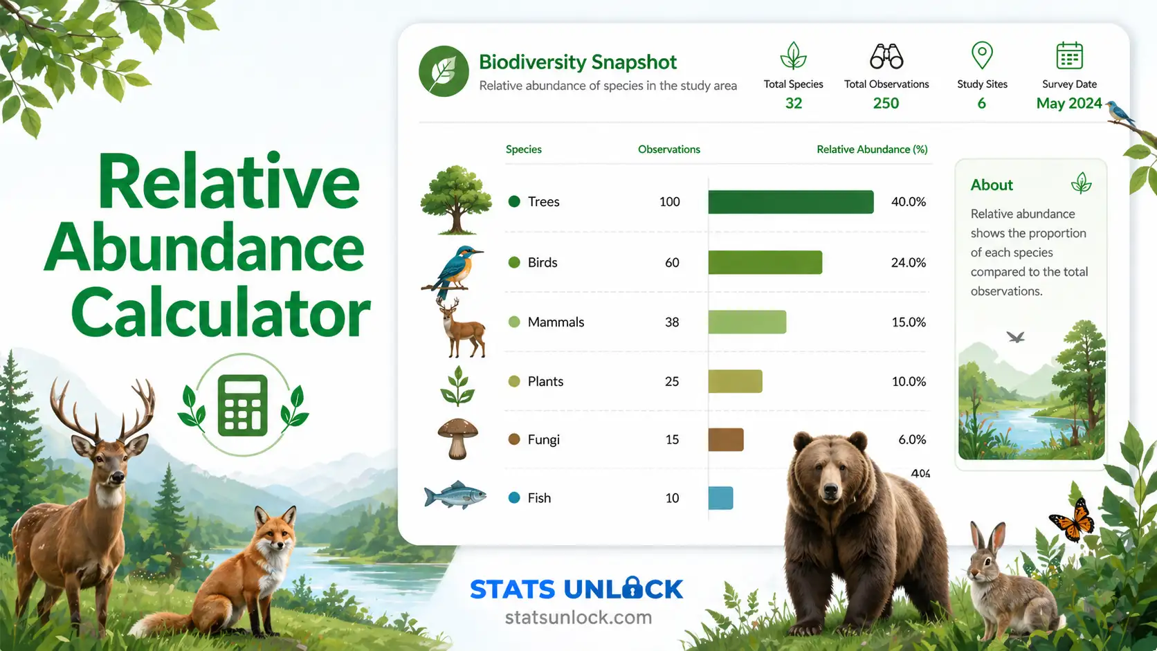

Relative Abundance Calculator
Enter species counts or isotope peaks and get the relative abundance of every item as a percentage, with rank, cumulative share, confidence intervals, dominance and evenness, four charts, and a ready-to-paste results sentence.
⚡ 0. Quick Answer
Relative abundance is the share of the total that belongs to one species or one isotope. Divide the count of that item by the total count of all items, then multiply by 100 to get a percentage.
If you count 100 birds and 40 are bulbuls, the relative abundance of the bulbul is 40%. The number tells you how common an item is compared with everything else in the same sample. It does not tell you how many there are in the area.
Rule of thumb: all relative abundances in one sample add up to 100%. A species above 50% dominates the community. A species below 1% is rare. In chemistry the same sum, taken over isotopes, is called percent abundance.
Key takeaways
- Relative abundance is a share: the count of one species or isotope divided by the total count, usually written as a percentage.
- It is a relative number, so it can go up for one species only because another species went down.
- Species richness counts how many species there are, and relative abundance says how the individuals are split between them.
- Small samples give wide confidence intervals, so always report the total count N beside each percentage.
- In chemistry, multiply each isotope mass by its fractional abundance and add the results to get the average atomic mass.
📚 1. What Is Relative Abundance?
Relative abundance is how common one thing is compared with all the other things counted in the same sample. In ecology the things are species and the sample is a community: a transect, a plot, a camera trap grid, or a water sample. In chemistry the things are the isotopes of one element. In microbiology they are the bacteria in a sequenced sample. The meaning is the same in every field: a part divided by the whole.
A simple definition: the relative abundance of a species is the number of individuals of that species divided by the total number of individuals of all species. Multiply by 100 and you have a percentage. Leave it as a fraction between 0 and 1 and you have a proportion, usually written pᵢ.
Where the number comes from. You need two things: a count for each species, written nᵢ, and the total of all counts, written N. Nothing else enters the formula. That is also its weakness. If the survey missed quiet or shy species, their share is too low and every other share is too high.
What relative abundance tells you. It tells you which species are common and which are rare, how evenly the individuals are shared out, and whether one species dominates. It lets you compare two sites that were sampled with different effort, because a percentage does not grow just because you walked a longer transect.
What it does not tell you. It does not tell you how many animals live in the area. That is absolute abundance, and it needs a method such as distance sampling or mark and recapture. A species can keep the same numbers and still fall in relative abundance when another species increases.
Why ecologists use it and not a simple count. Raw counts depend on effort. Two hours of survey will give more birds than one hour. Shares are much more stable, so they are the starting point for nearly every diversity index. Shannon, Simpson, Pielou and Berger-Parker all take the relative abundances pᵢ as their only input.
| Term | What it measures | Example |
|---|---|---|
| Relative abundance | Share of the total held by one species or isotope | 40 bulbuls out of 100 birds is 40% |
| Absolute abundance | The real number of individuals in an area | About 320 bulbuls live in the reserve |
| Species richness | How many different species were found | 6 species on the transect |
| Species evenness | How equal the relative abundances are | Pielou J′ of 0.85 is fairly even |
| Percent abundance | The chemistry name for the share of one isotope, summing to 100% | Chlorine-35 is 75.76% of chlorine atoms |
🧮 2. Set Up Your Data
Type a species name in the first column and its count for each site in the other columns. Empty cells are ignored. Each count column becomes one site.
📊 3. Results
🧠 4. Interpretation of Results, In Detail
4.1 What your relative abundance values say
The most abundant species at the study site is ___ with a relative abundance of ___%. The sample holds ___ individuals of ___ species.
4.2 Is one species dominating?
The Berger-Parker dominance value is ___, which means the commonest species holds ___% of all individuals. The top ___ species together make up 50% of the sample.
4.3 How evenly the individuals are shared
Pielou evenness is ___ and the Shannon index is ___. These two numbers summarise the whole list of relative abundances in one value each.
4.4 How far you can trust each percentage
With a total of ___ individuals, the ___% confidence interval for the commonest species runs from ___% to ___%. The rarest species was seen ___ times.
4.5 What relative abundance actually tells you
A relative abundance is a share of a sample. A value of 40% means that four in every ten individuals you recorded belong to that species. It is the plainest way to describe the structure of a community: which species are common, which are scarce, and how steeply the numbers fall from the first to the last.
Because it is a share, it is not tied to survey effort in the way a raw count is. Double the length of a transect and the counts roughly double, but the shares stay close to where they were. That is why relative abundance is the standard way to compare sites, seasons and studies that used different effort.
4.6 What does relative abundance not tell you?
It cannot tell you population size. A species with 40% relative abundance might be 40 birds or 40,000. It also cannot tell you whether a species truly increased. All the shares must add up to 100%, so when one species declines, the shares of all the others go up, even if their real numbers did not change at all. This is the main trap in reading relative abundance over time, and it is the reason microbiome studies now pair relative abundance with a measure of total load (Gloor et al., 2017; Vandeputte et al., 2017).
4.7 What is the difference between species richness and relative abundance?
Species richness is the number of species. Relative abundance is how the individuals are divided among those species. Two forests can each hold 20 species and still be very different places: one with every species at about 5%, the other with one species at 80% and nineteen species sharing the rest. Richness is the same. The relative abundance pattern is not. Together, richness and relative abundance are the two parts of species diversity, and a diversity index such as Shannon or Simpson combines both in one number (Hill, 1973).
4.8 What sampling does to the numbers
Small samples exaggerate. A species seen once in a sample of 20 gets a relative abundance of 5%, but its true share could be anywhere from about 1% to 24%. Rare species are also easy to miss completely, which pushes the shares of the common species upward. As a guide, you need about 300 individuals to have a 95% chance of recording a species whose true share is 1%.
Detection matters as much as sample size. Loud, bold or large species are recorded more often than quiet ones, so their relative abundance in the notebook is higher than in the forest. Camera trap studies meet the same problem, which is why a relative abundance index from photographs should be compared only within one study and one method (Sollmann et al., 2013).
4.9 What is the difference between percent abundance and relative abundance?
For isotopes the two terms are often used for the same thing, but they are not always the same number. Percent abundance is the share of all atoms of an element that are one isotope, and the values for all isotopes add up to 100%. On a mass spectrum, relative abundance is often plotted on a different scale, where the tallest peak, called the base peak, is set to 100 and every other peak is given as a percentage of it. Chlorine shows the difference well: its percent abundances are 75.76% and 24.24%, and the same data on a base-peak scale read 100 and 32.
Both scales describe the same ratio, about 3 to 1. To move from the base-peak scale to percent abundance, divide each peak by the sum of all peaks and multiply by 100. The chemistry mode of this calculator does that step for you and then works out the average atomic mass.
4.10 Practical judgement
Report each relative abundance with the total count N, so the reader can judge its precision. Do not rank species that differ by only a few individuals. Compare sites only when the same method, season and observer effort were used. When shares change between years, check the raw counts before you say that a species increased or declined. And remember that a relative abundance describes your sample first and the community second.
✍ 5. How to Write Your Results in Research
📌 Key conventions for this style
- Give N and S before any percentage.
- Use scientific names in italics at first mention.
- Report one decimal place unless N is above 1,000.
- Say how the confidence interval was calculated.
📌 Key conventions for this style
- Write the formula out in the methods chapter.
- State the survey method, effort and dates.
- Report dominance and evenness beside the species table.
- Put the full species table in an appendix.
📌 Key conventions for this style
- Say "out of every 100" and avoid symbols.
- Use common names only.
- Round to whole numbers.
- Explain that a share is not a population size.
📌 Key conventions for this style
- Keep to four labelled parts and under 250 words.
- Give the two or three most important percentages only.
- End with one clear take-home sentence.
- Replace the bracketed background line with your own study context.
📌 Key conventions for this style
- Use the same field order every year so reports can be compared.
- Record method, observer and effort with each entry.
- Keep the raw counts with the percentages.
- Flag any change in protocol clearly.
📌 Poster design notes
- Give the results block at least 40% of the poster area, with the bar chart as the main figure.
- Use A0 portrait (841 × 1189 mm) for conferences and A1 for seminars.
- Title at 72 pt or more, body text at 24 pt or more, so it reads from two metres away.
- Export charts at 300 dpi and keep to four colours or fewer.
∑ 6. Relative Abundance Formula: Formulas Used
🔀 7. Relative Abundance Calculation Flowchart, Step by Step
This flowchart shows how relative abundance is calculated, step by step, from raw field counts to the final verdict. Every box uses the same worked example as the Excel, R and Python sections: 100 birds of 6 species counted on one 2 km transect in dry deciduous forest.
Check any box yourself: the Excel sheet in Section 9, the R script in Section 10 and the Python script in Section 11 all return 40.0% for the bulbul, d = 0.400 and J′ = 0.851 for this dataset.
📝 8. How to Use This Calculator
- Choose what you are measuring. Leave the first button on Species counts for ecology data, or press Isotopes for chemistry. The two modes use the same formula but show different results.
- Enter your data. In the default tab, type or paste comma-separated entries such as
Bulbul: 40, Babbler: 25, Myna: 15. New lines, tabs and semicolons also work, so two columns pasted from Excel are fine. Plain numbers are accepted and are named Species 1, Species 2 and so on. - Name each site. The name box above every data box is editable. Type something useful such as Interior transect, March and it appears in the tables, the charts and the downloads.
- Add more sites to compare. Press Add site to compare two or more communities side by side. Each site gets its own percentages, and the calculator adds a comparison table and the percentage similarity between sites.
- Or upload a file. On the Upload tab, choose a CSV or Excel file, pick the column that holds the species names, and click every count column you want. Each column you click becomes one site.
- Try a sample dataset. Twelve built-in datasets cover an even forest community, a fragment dominated by one species, a tiny sample, a camera trap grid, a two-site comparison, microbiome reads and a messy field sheet.
- Fill in the study area name. This is optional. When you type it, the name is used in all five report sentences, the poster text, the conclusion and both downloads.
- Set the options. Choose what was counted, the number of decimal places, the confidence level, and the percentage below which a species is called rare.
- Press Calculate Relative Abundance. Nothing is calculated until you press the button. If you change any input afterwards, the results are cleared so you never read old numbers.
- Read the results and export. Check the summary cards and the full table, then the four charts. Sections 4, 5 and 18 fill in with your own numbers. Use Download Doc for a text report or Download PDF for a print-ready page.
📈 9. How to Calculate Relative Abundance in Excel
Excel has no function called relative abundance, but you do not need one. The whole calculation is one division. What goes wrong is the detail: a total that is not locked with dollar signs, a blank row that changes the total, and percentages that are formatted twice. This section shows the sheet at each stage, using the same six-species bird example as the rest of the page.
=B2/SUM($B$2:$B$7)*100 in C2, press Enter, and drag the formula down to C7. Column C is now the relative abundance of each species in percent.9.1 The functions you need
| You want | Excel function | Note |
|---|---|---|
| Total count, N | =SUM(B2:B7) | Blank cells are ignored |
| Relative abundance, % | =B2/$B$8*100 | The dollar signs lock the total when you fill down |
| Proportion, pᵢ | =B2/$B$8 | Use this form for diversity indices |
| Species richness, S | =COUNTIF(B2:B7,">0") | Counts only species that were seen |
| Rank | =RANK.EQ(C2,$C$2:$C$7) | 1 is the most abundant species |
| Berger-Parker dominance | =MAX(B2:B7)/B8 | Share of the commonest species, 0 to 1 |
| Shannon index | =-SUMPRODUCT(C2:C7/100,LN(C2:C7/100)) | Fails if any count is 0, see 9.3 |
| Pielou evenness | =B12/LN(B11) | Shannon index divided by ln S |
| Average atomic mass | =SUMPRODUCT(A2:A3,B2:B3)/SUM(B2:B3) | Isotope masses in A, abundances in B |
9.2 Step by step
1 Put species in column A and counts in column B
Type the species names down column A and the number of individuals beside each one in column B. Use one row per species. If a species is on two rows, add them together first.
The six species sit in A2:A7 and their counts in B2:B7. Cell B2 holds the 40 bulbuls.
2 Add up the total count
Click the cell under the last count and add the column. This is N, the number you will divide by.
=SUM(B2:B7)Cell B8 returns 100, the total number of birds on the transect.
3 Divide each count by the total and multiply by 100
In C2, divide the count by the total. Put dollar signs on the total so the reference does not move, then fill the formula down to the last species.
=B2/$B$8*100Column C shows 40, 25, 15, 10, 6 and 4. Cell C8 adds them to 100, which confirms that no row was left out.
4 Rank the species and build the cumulative share
Sort the table by column C, largest first. Then rank each species and add a running total so you can see how many species make up half of the community.
=RANK.EQ(C2,$C$2:$C$7)=SUM($C$2:C2)Column D gives ranks 1 to 6. Column E climbs 40, 65, 80, 90, 96, 100, so the top two species already hold 65% of all birds.
5 Add dominance, richness, Shannon and evenness
Four more cells turn the list of shares into the summary numbers that reviewers expect beside a relative abundance table.
=MAX(B2:B7)/B8=COUNTIF(B2:B7,">0")=-SUMPRODUCT(C2:C7/100,LN(C2:C7/100))=B12/LN(B11)The sheet returns Berger-Parker 0.400, richness 6, Shannon 1.525 and Pielou evenness 0.851, the same values as the flowchart in Section 7.
9.3 The awkward cases
Zero counts. A species with a count of 0 has a relative abundance of 0%, which is fine. The problem comes in the Shannon formula, because LN(0) returns an error. Wrap the log so that zero rows add nothing:
=-SUMPRODUCT(C2:C7/100,IFERROR(LN(C2:C7/100),0))
In Excel 2019 and earlier, confirm this formula with Ctrl + Shift + Enter. The classic mistake is to delete the zero row to make the error go away and then forget that the species was searched for and not found.
Several sites in one sheet. Put each site in its own column and divide by the total of that column, not by the grand total. With sites in B, C and D and totals in row 8:
=B2/B$8*100
Here only the row is locked, so the formula can be filled both down and across. Locking the column as well is the classic mistake, and it makes every site a share of site 1.
Isotopes and average atomic mass. With isotope masses in A2:A3 and their abundances in B2:B3, the average atomic mass is a weighted mean:
=SUMPRODUCT(A2:A3,B2:B3)/SUM(B2:B3)
For chlorine, masses 34.96885 and 36.96590 with abundances 75.76 and 24.24 return 35.453. Dividing by SUM(B2:B3) means the abundances can be percentages, fractions or peak heights. To go the other way and find the abundance of the lighter isotope from the average mass, use =(A3-B5)/(A3-A2) with the average mass in B5.
9.4 Why your Excel answer might differ from R or Python
| Situation | What happens | Fix |
|---|---|---|
| Blank cells in the count column | Excel ignores them, so N is smaller than you expect and every share is too high | Check that COUNT(B2:B7) equals the number of species |
| Zeros in the count column | They count as species in COUNT but not in the field, so richness is too high | Use COUNTIF(B2:B7,">0") for richness |
| Numbers stored as text | SUM skips them without a warning | Look for green triangles, then choose Convert to Number |
LN, LOG or LOG10 in the Shannon cell | LOG defaults to base 10 and gives 0.663, not 1.525 | Use LN to match this page, R and Python |
| Rounding shown, not stored | Shares shown as 33.3, 33.3, 33.3 seem to add to 99.9 | Excel still stores the full value, so the total is 100. Do not retype rounded numbers |
| Percent format plus × 100 | Values are shown 100 times too large | Remove the % format or remove *100 |
| Confidence intervals differ | A hand-built interval often uses the simple Wald formula | This page, R and Python use the Wilson interval, which is safer for rare species |
| Tool | Relative abundance, % | Shannon index |
|---|---|---|
| Excel | =B2/SUM($B$2:$B$7)*100 | =-SUMPRODUCT(p,LN(p)) |
| Google Sheets | =B2/SUM($B$2:$B$7)*100 | =-SUMPRODUCT(p,LN(p)) |
| R | counts / sum(counts) * 100 | -sum(p * log(p)) |
| Python NumPy | counts / counts.sum() * 100 | -(p * np.log(p)).sum() |
| Python pandas | df["count"] / df["count"].sum() * 100 | scipy.stats.entropy(df["count"]) |
9.5 Charting relative abundance in Excel
- Sort the table so the most abundant species is at the top.
- Select the species names and the relative abundance column.
- Choose Insert → Charts → Bar → Clustered Bar. A bar chart is easier to read than a pie chart once there are more than five species.
- Right-click the vertical axis, choose Format Axis and tick Categories in reverse order, so the commonest species sits at the top.
- Add the axis title Relative abundance (%) and put N in the chart title. A share without its sample size is the most common reason for a reviewer comment.
For a rank-abundance curve, plot rank on the horizontal axis and relative abundance on the vertical axis as a line chart, then set the vertical axis to a logarithmic scale. Chart 3 in Section 3 of this page draws it for you.
9.6 Excel errors you will probably hit
| Excel shows | Why | Fix |
|---|---|---|
#DIV/0! | The total cell is empty or 0 | Check the range in SUM and that counts are numbers |
#NUM! | LN was given a share of 0 | Wrap it as IFERROR(LN(...),0) |
#VALUE! | A count cell holds text such as "5+" or "many" | Replace it with a number, or leave the cell blank |
#N/A from RANK.EQ | The cell being ranked is outside the range you gave | Make the range cover every species and lock it with dollar signs |
| Shares do not add to 100 | The total was typed by hand, or the reference moved when filling down | Use $B$8 and recalculate the total with SUM |
| Every share is the same | Calculation is set to manual | Formulas → Calculation Options → Automatic |
📈 10. How to Calculate Relative Abundance in R
In R the relative abundance of a vector of counts is one line, counts / sum(counts) * 100. That line alone is rarely what you should report, because it gives no sample size, no precision and no summary of dominance. The script below is complete and runs from top to bottom. It calculates the relative abundance of every species with a Wilson confidence interval, adds dominance, the Shannon index and evenness, prints a plain-English verdict, and saves one publication-ready figure at 300 dpi.
Rscript, and it uses base R only, so there is nothing to install. Change only the counts <- c(...) line to use your own data.10.1 The complete script
R, base only, saves relative_abundance.png
# ============================================================
# Relative abundance of species, with one publication-ready plot
# StatsUnlock - https://statsunlock.com/relative-abundance-calculator/
# Base R only. No packages to install.
# ============================================================

# ---- 1. Your data ------------------------------------------
# Replace with your own counts, or read a CSV that has the
# columns "species" and "count":
#   dat    <- read.csv("counts.csv")
#   dat    <- dat[!is.na(dat$count), ]
#   counts <- setNames(dat$count, dat$species)
counts <- c(Bulbul = 40, Babbler = 25, Myna = 15,
            Robin = 10, Barbet = 6, Coucal = 4)

site <- "Dry deciduous forest transect"
conf <- 0.95

# ---- 2. Relative abundance ---------------------------------
counts <- sort(counts, decreasing = TRUE)   # most abundant first
N <- sum(counts)
if (N <= 0) stop("The total count is 0, so there is nothing to divide by.")
p   <- counts / N          # proportion, 0 to 1
ra  <- p * 100             # relative abundance, percent
cum <- cumsum(ra)          # cumulative share, percent

# ---- 3. Wilson confidence interval for each share ----------
z      <- qnorm(1 - (1 - conf) / 2)
den    <- 1 + z^2 / N
centre <- (p + z^2 / (2 * N)) / den
half   <- z * sqrt(p * (1 - p) / N + z^2 / (4 * N^2)) / den
lo     <- pmax(0, centre - half) * 100
hi     <- pmin(1, centre + half) * 100

# ---- 4. Dominance, diversity and evenness ------------------
pp      <- p[p > 0]                 # leave out zero counts before the log
S       <- length(pp)               # species richness
d       <- max(p)                   # Berger-Parker dominance
H       <- -sum(pp * log(pp))       # Shannon index, natural log
J       <- if (S > 1) H / log(S) else NA   # Pielou evenness
simpson <- 1 - sum(pp^2)            # Simpson diversity, 1 - D

# ---- 5. Printed summary ------------------------------------
tab <- data.frame(species       = names(counts),
                  count         = as.numeric(counts),
                  rel_abund_pct = round(as.numeric(ra), 2),
                  cum_pct       = round(as.numeric(cum), 2),
                  ci_low        = round(as.numeric(lo), 1),
                  ci_high       = round(as.numeric(hi), 1))
cat(sprintf("Site: %s\n", site))
cat(sprintf("Total individuals N = %d, species richness S = %d\n", as.integer(N), S))
print(tab, row.names = FALSE)
cat(sprintf("Berger-Parker d = %.3f\n", d))
cat(sprintf("Shannon H' = %.3f, Pielou J' = %.3f, Simpson 1-D = %.3f\n", H, J, simpson))

verdict <- if (d >= 0.50) {
  "one species holds half or more of all individuals, so dominance is high"
} else if (d >= 0.25) {
  "the commonest species is clearly ahead but does not hold the majority, so dominance is moderate"
} else {
  "no species stands far above the others, so dominance is low"
}
cat(sprintf("Verdict: %s is the most abundant species at %.1f%%, and %s.\n",
            names(counts)[1], ra[1], verdict))

# ---- 6. One figure, 300 dpi --------------------------------
colours <- c("#16a34a", "#2563eb", "#ea580c", "#9333ea", "#ca8a04",
             "#0d9488", "#db2777", "#475569", "#0891b2", "#b45309")
bar_cols <- rep(colours, length.out = length(counts))

png("relative_abundance.png", width = 3000, height = 1350, res = 300)
par(mfrow = c(1, 2), mar = c(4.5, 6.5, 3, 1.5))

# Left panel: sorted bars with confidence intervals
bp <- barplot(rev(as.numeric(ra)), horiz = TRUE, names.arg = rev(names(counts)),
              las = 1, col = rev(bar_cols), border = "white",
              xlim = c(0, max(hi) * 1.22),
              xlab = "Relative abundance (%)",
              main = sprintf("Share of each species (N = %d)", as.integer(N)))
arrows(rev(lo), bp, rev(hi), bp, angle = 90, code = 3, length = 0.04)
text(rev(hi) + 1, bp, sprintf("%.1f%%", rev(ra)), adj = 0, cex = 0.8)

# Right panel: rank-abundance curve on a log scale
par(mar = c(4.5, 4.5, 3, 1))
plot(seq_len(S), ra[seq_len(S)], log = "y", type = "b", pch = 19,
     col = "#2563eb", lwd = 2, xaxt = "n",
     xlab = "Species rank (1 = most abundant)",
     ylab = "Relative abundance (%), log scale",
     main = sprintf("Rank-abundance curve (J' = %.2f)", J))
axis(1, at = seq_len(S))
grid()

dev.off()
cat("Saved relative_abundance.png\n")
10.2 What each part does
| Line or function | What it does and why it is there |
|---|---|
| counts <- c(...) | A named numeric vector: each name is a species and each value is its count. Swap in the commented read.csv() lines to load a file. The line with !is.na() drops missing counts, because one NA would turn the total and every share into NA. |
| sort(counts, decreasing = TRUE) | Puts the most abundant species first, which is the order used in the table, the bars and the rank-abundance curve. |
| counts / N | R divides the whole vector at once, so every species gets its proportion in one step. Multiplying by 100 gives the relative abundance in percent. |
| cumsum(ra) | The running total of the shares. It shows how many species are needed to reach 50% or 90% of the community. |
| qnorm() | Turns the confidence level into the z value: 1.960 for 95%. Change conf to 0.90 or 0.99 to change the interval. |
| centre, half | The Wilson interval. It is preferred to the simple formula because it never goes below 0% or above 100% and behaves well for rare species. |
| p[p > 0] | Removes zero counts before the logarithm. log(0) is -Inf in R and 0 * -Inf is NaN, which would spoil the Shannon index. |
| log(pp) | R's log() is the natural log. Some ecology papers use log2() or log10(), which gives a different Shannon value from the same data. Say which base you used. |
| data.frame(...) | Builds the results table. as.numeric() strips the species names from each column so they are not printed twice. |
| sprintf() | Formats numbers to a fixed number of decimals. %.3f is three decimals, %d is a whole number and %% prints a percent sign. |
| png(..., res = 300) | Opens a file to draw into at print quality. Without res = 300 the image is 72 dpi and looks blurred in a thesis or paper. |
| barplot(rev(...), horiz = TRUE) | Horizontal bars are drawn from the bottom up, so the vectors are reversed with rev() to put the commonest species at the top. |
| arrows(..., angle = 90, code = 3) | Draws the confidence interval as an error bar with a flat cap at each end. |
| plot(..., log = "y") | The rank-abundance curve. The log scale stops the common species from hiding the pattern among the rare ones. |
| dev.off() | Closes the file. If you forget it the PNG is empty or locked, which is the most common plotting problem in R. |
10.3 What the figure shows
The left panel is a sorted bar chart of relative abundance with one bar per species and a thin error bar for the 95% confidence interval. Bars whose error bars overlap a lot should not be ranked against each other with confidence. The right panel is the rank-abundance curve on a log scale. A steep fall from rank 1 to rank 2 means one species dominates. A gentle slope means the individuals are shared evenly. For the example data the line falls steadily from 40% to 4%, which matches the moderate dominance and high evenness in the printed verdict.
10.4 Common R problems and fixes
| Symptom | Cause | Fix |
|---|---|---|
Every share is NA | One count is missing, so sum() returns NA | Drop missing rows first, or use sum(counts, na.rm = TRUE) |
Shannon index is NaN | A count of 0 reached log() | Use pp <- p[p > 0] as in the script |
non-numeric argument to binary operator | The count column was read as text | Convert with as.numeric() and check for stray characters such as "5+" |
| Species names are missing from the plot | The vector has no names | Build it with setNames(dat$count, dat$species) |
| Long names are cut off on the left | The left margin is too small | Raise the second number in par(mar = ...), for example to 10 |
| The PNG is empty | dev.off() was not run | Run while (dev.cur() > 1) dev.off() and then the script again |
vegan::decostand gives different numbers | It works on rows, and your species are in rows not columns | Put sites in rows and species in columns, or use MARGIN = 2 |
| Warning about zero-length arrows | A species has an interval too short to draw | Safe to ignore, the bar is still correct |
10.5 Useful one-liners
| You want | R code |
|---|---|
| Relative abundance in percent | counts / sum(counts) * 100 |
| The same, from raw observations | prop.table(table(obs$species)) * 100 |
| Every site at once, sites in rows | prop.table(as.matrix(m), margin = 1) * 100 |
| With the vegan package | vegan::decostand(m, method = "total") * 100 |
| Wilson interval for one species | prop.test(40, 100, correct = FALSE)$conf.int * 100 |
| Berger-Parker dominance | max(counts) / sum(counts) |
| Percentage similarity of two sites | sum(pmin(ra1, ra2)) |
| Average atomic mass | weighted.mean(c(34.96885, 36.96590), c(75.76, 24.24)) |
| Save the table | write.csv(tab, "relative_abundance.csv", row.names = FALSE) |
📈 11. How to Calculate Relative Abundance in Python
Python gives the relative abundance in one line as well, counts / counts.sum() * 100, and it carries the same risk of being reported with nothing beside it. The script below is complete and runnable. It calculates the share of every species with a Wilson confidence interval, adds dominance, the Shannon index and evenness, prints a verdict in plain English, and saves one 300 dpi figure ready for a paper or a slide.
species = [...] and counts = np.array([...]) lines.Install with pip install numpy matplotlib if you do not already have them. Add pandas only if you use the commented CSV lines.
11.1 The complete script
Python, numpy and matplotlib, saves relative_abundance.png
# ============================================================
# Relative abundance of species, with one publication-ready plot
# StatsUnlock - https://statsunlock.com/relative-abundance-calculator/
# Needs numpy and matplotlib only.
# ============================================================
import numpy as np
import matplotlib.pyplot as plt

# ---- 1. Your data ------------------------------------------
# Replace these two lines with your own species and counts,
# or read a CSV that has the columns "species" and "count":
#   import pandas as pd
#   df = pd.read_csv("counts.csv").dropna(subset=["count"])
#   species = df["species"].tolist()
#   counts = df["count"].to_numpy(dtype=float)
species = ["Bulbul", "Babbler", "Myna", "Robin", "Barbet", "Coucal"]
counts = np.array([40, 25, 15, 10, 6, 4], dtype=float)

site = "Dry deciduous forest transect"
z = 1.959964          # 1.644854 for 90%, 2.575829 for 99%

# ---- 2. Relative abundance ---------------------------------
order = np.argsort(-counts, kind="stable")      # most abundant first
species = [species[i] for i in order]
counts = counts[order]

N = counts.sum()
if N <= 0:
    raise SystemExit("The total count is 0, so there is nothing to divide by.")
p = counts / N                 # proportion, 0 to 1
ra = p * 100                   # relative abundance, percent
cum = np.cumsum(ra)            # cumulative share, percent

# ---- 3. Wilson confidence interval for each share ----------
den = 1 + z**2 / N
centre = (p + z**2 / (2 * N)) / den
half = z * np.sqrt(p * (1 - p) / N + z**2 / (4 * N**2)) / den
lo = np.clip(centre - half, 0, 1) * 100
hi = np.clip(centre + half, 0, 1) * 100

# ---- 4. Dominance, diversity and evenness ------------------
pp = p[p > 0]                  # leave out zero counts before the log
S = int(pp.size)               # species richness
d = p.max()                    # Berger-Parker dominance
H = -(pp * np.log(pp)).sum()   # Shannon index, natural log
J = H / np.log(S) if S > 1 else float("nan")   # Pielou evenness
simpson = 1 - (pp**2).sum()    # Simpson diversity, 1 - D

# ---- 5. Printed summary ------------------------------------
print(f"Site: {site}")
print(f"Total individuals N = {N:.0f}, species richness S = {S}")
print(f"{'Species':<12}{'Count':>7}{'RA %':>9}{'Cum %':>9}{'95% CI':>16}")
for s, n, r, c, a, b in zip(species, counts, ra, cum, lo, hi):
    print(f"{s:<12}{n:>7.0f}{r:>9.2f}{c:>9.2f}{a:>9.1f} to {b:<5.1f}")
print(f"Berger-Parker d = {d:.3f}")
print(f"Shannon H' = {H:.3f}, Pielou J' = {J:.3f}, Simpson 1-D = {simpson:.3f}")

if d >= 0.50:
    verdict = "one species holds half or more of all individuals, so dominance is high"
elif d >= 0.25:
    verdict = "the commonest species is clearly ahead but does not hold the majority, so dominance is moderate"
else:
    verdict = "no species stands far above the others, so dominance is low"
print(f"Verdict: {species[0]} is the most abundant species at {ra[0]:.1f}%, and {verdict}.")

# ---- 6. One figure, 300 dpi --------------------------------
colours = ["#16a34a", "#2563eb", "#ea580c", "#9333ea", "#ca8a04", "#0d9488",
           "#db2777", "#475569", "#0891b2", "#b45309"]
bar_cols = [colours[i % len(colours)] for i in range(len(species))]

fig, (ax1, ax2) = plt.subplots(1, 2, figsize=(10, 4.4))

ypos = np.arange(len(species))[::-1]
ax1.barh(ypos, ra, color=bar_cols, edgecolor="white")
ax1.errorbar(ra, ypos, xerr=[ra - lo, hi - ra], fmt="none", ecolor="#111827",
             elinewidth=1, capsize=3)
ax1.set_yticks(ypos)
ax1.set_yticklabels(species)
ax1.set_xlabel("Relative abundance (%)")
ax1.set_title(f"Share of each species (N = {N:.0f})")
for y, r, h in zip(ypos, ra, hi):
    ax1.text(h + 1, y, f"{r:.1f}%", va="center", fontsize=9)
ax1.set_xlim(0, hi.max() * 1.22)

rank = np.arange(1, S + 1)
ax2.plot(rank, ra[:S], marker="o", color="#2563eb", linewidth=1.8)
ax2.set_yscale("log")
ax2.set_xticks(rank)
ax2.set_xlabel("Species rank (1 = most abundant)")
ax2.set_ylabel("Relative abundance (%), log scale")
ax2.set_title(f"Rank-abundance curve (J' = {J:.2f})")
ax2.grid(True, which="both", linewidth=0.4, alpha=0.5)

fig.suptitle(site, fontsize=11, y=1.02)
fig.tight_layout()
fig.savefig("relative_abundance.png", dpi=300, bbox_inches="tight")
print("Saved relative_abundance.png")
11.2 What each part does
| Line or function | What it does and why it is there |
|---|---|
| np.array([...], dtype=float) | Stores the counts as decimals. Without dtype=float some older setups do whole-number division and return 0 for every share. |
| pd.read_csv(...).dropna() | The optional file route. dropna removes rows with no count, because one nan makes the total and every share nan. |
| np.argsort(-counts, kind="stable") | Gives the order from largest to smallest count. kind="stable" keeps tied species in the order you typed them. |
| counts / N | NumPy divides the whole array at once. Multiplying by 100 gives relative abundance in percent. |
| np.cumsum(ra) | The running total of the shares, used for the cumulative column. |
| centre, half | The Wilson interval, the same formula as the R script and the calculator on this page. |
| np.clip(..., 0, 1) | Keeps the interval between 0% and 100% against tiny rounding errors. |
| p[p > 0] | Removes zero counts before the logarithm. np.log(0) is -inf and raises a warning. |
| np.log(pp) | The natural log. Use np.log2 or np.log10 only if the paper you compare with did the same. |
| f"{r:>9.2f}" | An f-string format: right-aligned, nine characters wide, two decimals. This is what lines the printed table up in columns. |
| ax1.barh(...) | Horizontal bars. The positions are reversed with [::-1] so that the commonest species is at the top. |
| ax1.errorbar(..., fmt="none") | Draws only the error bars, on top of the bars, for the confidence interval. |
| ax2.set_yscale("log") | Puts the rank-abundance curve on a log scale so that rare species can still be read. |
| fig.savefig(..., dpi=300, bbox_inches="tight") | Saves at print quality and trims empty white space around the figure. |
11.3 What the figure shows
The figure has the same two panels as the R version. On the left are the sorted bars with 95% confidence intervals and a percentage label at the end of each bar. On the right is the rank-abundance curve on a log scale, with Pielou evenness in the title. Read the left panel to see which species are common. Read the right panel to see the shape of the community: steep means dominated, flat means even.
11.4 Common Python problems and fixes
| Symptom | Cause | Fix |
|---|---|---|
Every share is nan | One count is nan | Drop missing rows, or use np.nansum(counts) for the total |
RuntimeWarning: divide by zero encountered in log | A zero share reached np.log | Filter with pp = p[p > 0] first |
| Every share is 0 | Whole-number division in an old Python or NumPy | Create the array with dtype=float |
scipy.stats.entropy gives a different number | It was given a different log base, or raw counts that it normalised itself | It normalises its input, so pass counts directly and leave base unset for natural log |
ModuleNotFoundError | NumPy or Matplotlib is not installed in this environment | Run pip install numpy matplotlib in the same environment |
| Labels are cut off in the saved file | The figure was saved without tight bounding | Keep bbox_inches="tight" |
| No window opens | The script saves to file and does not call plt.show() | Open relative_abundance.png, or add plt.show() at the end |
| pandas shares do not add to 100 | Duplicate species rows were not merged | Use df.groupby("species")["count"].sum() first |
11.5 Useful one-liners
| You want | Python code |
|---|---|
| Relative abundance in percent | counts / counts.sum() * 100 |
| From raw observations, pandas | df["species"].value_counts(normalize=True) * 100 |
| Every site at once, sites in rows | m.div(m.sum(axis=1), axis=0) * 100 |
| Berger-Parker dominance | counts.max() / counts.sum() |
| Shannon index with SciPy | scipy.stats.entropy(counts) |
| Wilson interval with statsmodels | proportion_confint(40, 100, method="wilson") |
| Percentage similarity of two sites | np.minimum(ra1, ra2).sum() |
| Average atomic mass | np.average([34.96885, 36.96590], weights=[75.76, 24.24]) |
Run it from a terminal with python relative_abundance.py. In Jupyter, delete the savefig line and add plt.show() to see the figure under the cell.
📋 12. Reference Tables
12.1 Relative abundance and the terms it is confused with
| Term | Formula | What it answers |
|---|---|---|
| Relative abundance | (nᵢ ÷ N) × 100 | What share of all individuals is this species? |
| Absolute abundance | Estimated number of individuals | How many are there in the area? |
| Density | Individuals ÷ area | How many per hectare or per square kilometre? |
| Species richness | S = number of species | How many different species are there? |
| Relative frequency | (Plots with species ÷ sum for all species) × 100 | How widely is the species spread across plots? |
| Relative abundance index, RAI | (Independent photo events ÷ trap nights) × 100 | How often is the species photographed per 100 trap nights? |
| Percent abundance, chemistry | (Atoms of isotope ÷ all atoms of element) × 100 | What share of the atoms is this isotope? |
Conclusion: relative abundance is always a share of a total. If the number you have is divided by area or by effort, it is a density or a rate, not a relative abundance. The camera trap RAI is a rate per unit effort and its values do not add up to 100 (O'Brien et al., 2003).
12.2 Working bands used by this calculator
| Measure | Value | Label on this page |
|---|---|---|
| Berger-Parker dominance, d | 0.50 or more | High dominance one species holds half or more |
| 0.25 to 0.49 | Moderate dominance | |
| Below 0.25 | Low dominance | |
| Pielou evenness, J′ | 0.70 or more | High evenness |
| 0.40 to 0.69 | Moderate evenness | |
| Below 0.40 | Low evenness | |
| Total count, N | 100 or more | Adequate sample |
| 30 to 99 | Small sample | |
| Below 30 | Very small sample |
Conclusion: these bands are working rules for this tool, chosen so that the labels are easy to read. They are not a published standard. Dominance and evenness depend on the habitat and the group studied, so compare your values with other studies of the same kind before you call a community dominated (Berger & Parker, 1970; Hill, 1973).
12.3 How precise is one relative abundance? 95% Wilson intervals
| Total count, N | Share of 5% | Share of 10% | Share of 25% | Share of 50% |
|---|---|---|---|---|
| 20 | 0.9 to 23.6 | 2.8 to 30.1 | 11.2 to 46.9 | 29.9 to 70.1 |
| 100 | 2.2 to 11.2 | 5.5 to 17.4 | 17.5 to 34.3 | 40.4 to 59.6 |
| 400 | 3.3 to 7.6 | 7.4 to 13.3 | 21.0 to 29.5 | 45.1 to 54.9 |
| 1,000 | 3.8 to 6.5 | 8.3 to 12.0 | 22.4 to 27.8 | 46.9 to 53.1 |
Conclusion: at N = 20 a share of 25% could really be anything from about 11% to 47%. At N = 1,000 the same share is known to within about 3 percentage points. Precision depends on N far more than on the share itself (Wilson, 1927).
12.4 How many individuals you need to record a rare species
| True relative abundance of the species | Individuals needed for a 95% chance of at least one record | Formula check |
|---|---|---|
| 20% | 14 | ln 0.05 ÷ ln 0.80 |
| 10% | 29 | ln 0.05 ÷ ln 0.90 |
| 5% | 59 | ln 0.05 ÷ ln 0.95 |
| 2% | 149 | ln 0.05 ÷ ln 0.98 |
| 1% | 299 | ln 0.05 ÷ ln 0.99 |
| 0.1% | 2,995 | ln 0.05 ÷ ln 0.999 |
Conclusion: a sample of 100 individuals will often miss species below about 3%. Missing species make the shares of the recorded species look larger than they are, which is why richness and relative abundance from small samples must be read with care (Gotelli & Colwell, 2001; Preston, 1948).
12.5 Natural percent abundance of common isotopes
| Element | Isotope | Mass (u) | Percent abundance | Average atomic mass (u) |
|---|---|---|---|---|
| Hydrogen | ¹H | 1.00783 | 99.9885 | 1.008 |
| ²H | 2.01410 | 0.0115 | ||
| Lithium | ⁶Li | 6.01512 | 7.59 | 6.94 |
| ⁷Li | 7.01600 | 92.41 | ||
| Boron | ¹⁰B | 10.01294 | 19.9 | 10.81 |
| ¹¹B | 11.00931 | 80.1 | ||
| Carbon | ¹²C | 12.00000 | 98.93 | 12.011 |
| ¹³C | 13.00335 | 1.07 | ||
| Magnesium | ²⁴Mg | 23.98504 | 78.99 | 24.305 |
| ²⁵Mg | 24.98584 | 10.00 | ||
| ²⁶Mg | 25.98259 | 11.01 | ||
| Chlorine | ³⁵Cl | 34.96885 | 75.76 | 35.45 |
| ³⁷Cl | 36.96590 | 24.24 | ||
| Copper | ⁶³Cu | 62.92960 | 69.15 | 63.546 |
| ⁶⁵Cu | 64.92779 | 30.85 | ||
| Bromine | ⁷⁹Br | 78.91834 | 50.69 | 79.904 |
| ⁸¹Br | 80.91629 | 49.31 |
Conclusion: these are the representative values in the IUPAC tables (Meija et al., 2016a, 2016b). Natural samples vary a little, which is why the atomic mass of some elements is now given as a range. Use the values your textbook or exam board gives if they differ in the last digit.
12.6 The same data on three scales
| Item | Raw value | Proportion (0 to 1) | Percent (sums to 100) | Base peak = 100 |
|---|---|---|---|---|
| Bulbul | 40 birds | 0.40 | 40.0 | 100.0 |
| Babbler | 25 birds | 0.25 | 25.0 | 62.5 |
| Myna | 15 birds | 0.15 | 15.0 | 37.5 |
| Chlorine-35 | peak height 100 | 0.7576 | 75.76 | 100.0 |
| Chlorine-37 | peak height 32 | 0.2424 | 24.24 | 32.0 |
Conclusion: proportion and percent are the same number with the decimal point moved. The base-peak scale is different: it divides by the largest value, not by the total, so it does not add up to 100. Always say which scale a relative abundance is on.
12.7 What relative abundance is a share of, by field
| Field | What is counted | The total, N | Main caution |
|---|---|---|---|
| Bird and mammal surveys | Individuals seen or heard | All individuals of all species | Species differ in how easy they are to detect |
| Camera trapping | Independent photo events | All events of all species | Events are not individuals, and large species trigger cameras more often |
| Vegetation plots | Stems, cover or basal area | Sum over all species | Say which measure was used, because the three give different shares |
| Microbiome sequencing | Sequence reads per taxon | All reads in the sample | The total is set by the machine, so shares are compositional |
| Chemistry, isotopes | Atoms, or ion signal on a mass spectrum | All isotopes of one element | Check whether the scale is percent or base peak |
Conclusion: the formula never changes, but the meaning of the total does. For sequence reads the total carries no biological meaning at all, so a rise in one taxon forces a fall in the others (Gloor et al., 2017; Vandeputte et al., 2017).
📈 13. Example Results
Six bird species on a dry forest transect
The clean case used in every worked example on this page.
An observer walks a 2 km transect in dry deciduous forest and records 100 birds of six species.
| Measure | Value | Note |
|---|---|---|
| Total count, N | 100 | All individuals in the sample |
| Species richness, S | 6 | Species with a count above 0 |
| Bulbul | 40.0% | 40 of 100, 95% CI 30.9 to 49.8% |
| Babbler | 25.0% | 25 of 100, 95% CI 17.5 to 34.3% |
| Myna | 15.0% | 15 of 100, 95% CI 9.3 to 23.3% |
| Berger-Parker d | 0.400 | Share of the commonest species |
| Pielou evenness J′ | 0.851 | 1 means perfectly even |
| Shannon H′ | 1.525 | Natural log, in nats |
What it means: Four in every ten birds were bulbuls, and the top two species together make up 65% of the count. Dominance is moderate and evenness is high, so this is a mixed community with one clear leader, not a community controlled by one species.
How to write it: "We recorded 100 birds of six species. The bulbul was the most abundant (40.0%, 95% CI 30.9 to 49.8%), followed by the babbler (25.0%). Berger-Parker dominance was 0.40 and Pielou evenness 0.85."
Wet evergreen forest point counts
Many species, and none of them far ahead.
Twelve point counts in wet evergreen forest give 110 birds of 12 species.
| Measure | Value | Note |
|---|---|---|
| Total count, N | 110 | All individuals in the sample |
| Species richness, S | 12 | Species with a count above 0 |
| Yellow-browed Bulbul | 12.7% | 14 of 110, 95% CI 7.7 to 20.2% |
| Malabar Barbet | 11.8% | 13 of 110, 95% CI 7.0 to 19.2% |
| Crimson-backed Sunbird | 10.9% | 12 of 110, 95% CI 6.4 to 18.1% |
| Berger-Parker d | 0.127 | Share of the commonest species |
| Pielou evenness J′ | 0.972 | 1 means perfectly even |
| Shannon H′ | 2.415 | Natural log, in nats |
What it means: No species holds more than 13% of the birds. Evenness is 0.97, close to the maximum of 1. The ranking of the top five species should not be trusted, because their intervals overlap almost completely. The honest summary is that the community is very even.
How to write it: "Relative abundance was similar across species (range 2.7 to 12.7%, N = 110, S = 12), with low dominance (d = 0.13) and very high evenness (J′ = 0.97)."
Logged forest fragment
One generalist holds two thirds of the count.
A transect through a logged fragment next to a village gives 200 birds of 7 species.
| Measure | Value | Note |
|---|---|---|
| Total count, N | 200 | All individuals in the sample |
| Species richness, S | 7 | Species with a count above 0 |
| House Crow | 66.0% | 132 of 200, 95% CI 59.2 to 72.2% |
| Common Myna | 14.0% | 28 of 200, 95% CI 9.9 to 19.5% |
| Red-vented Bulbul | 7.0% | 14 of 200, 95% CI 4.2 to 11.4% |
| Berger-Parker d | 0.660 | Share of the commonest species |
| Pielou evenness J′ | 0.604 | 1 means perfectly even |
| Shannon H′ | 1.174 | Natural log, in nats |
What it means: Two in every three birds are house crows. Seven species are present, which sounds reasonable, but richness hides how little of the community the other six make up. This is why relative abundance should always be reported beside richness.
How to write it: "The fragment was dominated by the house crow (66.0%, 95% CI 59.2 to 72.2%; N = 200). The six other species together made up 34.0% of individuals (d = 0.66, J′ = 0.60)."
A single short point count
The percentages look precise. They are not.
One 10 minute point count on a windy morning gives only 18 birds of 5 species.
| Measure | Value | Note |
|---|---|---|
| Total count, N | 18 | All individuals in the sample |
| Species richness, S | 5 | Species with a count above 0 |
| Bulbul | 38.9% | 7 of 18, 95% CI 20.3 to 61.4% |
| Babbler | 27.8% | 5 of 18, 95% CI 12.5 to 50.9% |
| Myna | 16.7% | 3 of 18, 95% CI 5.8 to 39.2% |
| Berger-Parker d | 0.389 | Share of the commonest species |
| Pielou evenness J′ | 0.886 | 1 means perfectly even |
| Shannon H′ | 1.426 | Natural log, in nats |
What it means: The shares are close to those in Example 1, but with 18 birds they carry very little weight. The bulbul could hold a fifth of the community or well over half. Species below about 15% were quite likely to be missed. Collect more counts before ranking anything.
How to write it: "Only 18 individuals were recorded, so relative abundances are reported for description only (bulbul 38.9%, 95% CI 20.3 to 61.4%)."
Forest interior against forest edge
Same six species, very different shares.
Two transects of equal length, one inside the forest and one along its edge, give 100 birds each.
| Species | Interior | Edge |
|---|---|---|
| Bulbul | 22.0% | 45.0% |
| Babbler | 30.0% | 15.0% |
| Myna | 4.0% | 28.0% |
| Robin | 12.0% | 6.0% |
| Barbet | 20.0% | 4.0% |
| Coucal | 12.0% | 2.0% |
| Pielou evenness J′ | 0.923 | 0.768 |
| Percentage similarity | 53.0% | Sum of the smaller share for each species |
What it means: Richness is 6 at both sites, so a richness comparison would show no difference at all. The relative abundances tell the real story: the myna rises from 4% to 28% at the edge and the barbet falls from 20% to 4%. Percentage similarity is only 53%.
How to write it: "Species richness was the same at both sites (S = 6), but composition differed (percentage similarity = 53.0%). The myna made up 4.0% of birds in the interior and 28.0% at the edge."
Wetland waterbirds in 2022 and 2025
A share can fall while the count barely moves.
The same wetland is counted in two winters. The total is 600 birds in both years.
| Species | Winter 2022 | Winter 2025 |
|---|---|---|
| Northern Pintail | 180 birds, 30.0% | 90 birds, 15.0% |
| Common Teal | 150 birds, 25.0% | 160 birds, 26.7% |
| Eurasian Coot | 120 birds, 20.0% | 260 birds, 43.3% |
| Bar-headed Goose | 90 birds, 15.0% | 50 birds, 8.3% |
| Little Grebe | 60 birds, 10.0% | 40 birds, 6.7% |
| Berger-Parker d | 0.300 | 0.433 |
What it means: The coot rose from 120 to 260 birds and the pintail halved from 180 to 90. Here the totals happen to be equal, so shares and counts agree. If the total had changed, a species could lose share without losing a single bird, so always read the counts beside the percentages.
How to write it: "Between 2022 and 2025 the relative abundance of Eurasian coot rose from 20.0% to 43.3% and that of northern pintail fell from 30.0% to 15.0% (N = 600 in both years)."
Duplicates, a zero and a blank
What the calculator does with untidy data.
A field sheet lists the bulbul twice (12 and 8), a myna with a count of 0, a robin with no number, and a koel recorded as "many".
| Species | Count used | Relative abundance |
|---|---|---|
| Bulbul | 20 | 40.0% |
| Babbler | 15 | 30.0% |
| Unidentified | 10 | 20.0% |
| Barbet | 5 | 10.0% |
| Myna | 0 | 0.0% |
| Robin, Koel | not readable | left out and reported |
What it means: The calculator merges rows with the same name, keeps the zero, and tells you which entries it could not read. The 10 unidentified birds stay in the total, which lowers every other share. Decide on purpose whether to keep them, and say what you did.
How to write it: "Ten unidentified individuals (20.0%) were retained in the total. Two entries without a numeric count were excluded."
Chlorine isotopes and average atomic mass
The same formula, applied to atoms.
A mass spectrum of chlorine atoms shows two peaks: mass 35 with a height of 100 and mass 37 with a height of 32.
| Isotope | Mass (u) | Peak height | Percent abundance |
|---|---|---|---|
| Chlorine-35 | 34.96885 | 100 | 75.76% |
| Chlorine-37 | 36.96590 | 32 | 24.24% |
| Average atomic mass | 35.453 u |
What it means: Dividing each peak by the total of 132 gives 75.76% and 24.24%. Multiplying each mass by its fraction and adding gives 35.453 u, the value in the periodic table. The same 3 to 1 pattern appears in the mass spectrum of any compound with one chlorine atom.
How to write it: "Chlorine consists of 75.76% chlorine-35 and 24.24% chlorine-37, giving an average atomic mass of 34.96885 × 0.7576 + 36.96590 × 0.2424 = 35.453 u."
🧪 14. How to Collect Raw Data in the Field
Study design: relative abundance needs one count per species from one defined sample, collected with the same method and effort for every species. The eighteen points below take you from planning to a clean data sheet.
Plan
- Decide what your relative abundance will be a share of. Write down the group (for example all diurnal birds), the area and the season before you start. A share has no meaning without its total.
- Choose one method and keep it. Use point counts of 10 minutes with a 50 m radius, line transects of 1 to 2 km, or 20 m × 20 m vegetation plots. Do not mix methods inside one sample.
- Plan for at least 100 individuals per site. Below 30 individuals the confidence intervals are too wide to rank species. Add points or repeat visits until you reach the target.
- Spread the sampling units. Place points at least 250 m apart and transects at least 500 m apart so that the same bird is not counted twice.
- Fix the time window. Count birds from sunrise to about 3 hours after sunrise. Run camera traps for at least 30 days per station. Keep the same window at every site.
Kit
- Carry a printed data sheet with one row per species. Add columns for site, date, start time, observer, weather and tally marks. Pre-print the expected species to speed up recording.
- Use binoculars of 8 × 42 and a rangefinder. The rangefinder lets you check the 50 m radius, which stops distant loud species from inflating their share.
- Record position with a GPS unit or phone. Save every point or transect start and end to within 5 m, so the survey can be repeated.
- Bring a regional field guide and a sound recorder. Record unknown calls and identify them later. Do not guess in the field.
- Carry a tally counter for flocks. Large flocks are the biggest source of counting error, and one flock can change every relative abundance on the sheet.
Collect
- Count individuals, not sightings. If the same bird is seen three times, it is one individual. For camera traps, treat photos of one species at one station within 30 minutes as one event.
- Collect the species counts for relative abundance in one pass. Record every individual of every species in the group. Do not skip common species because they are boring: they are the largest part of the total.
- Write unidentified individuals on their own row. Label them "Unidentified warbler", not as a guess. Decide later whether to keep them in the total.
- Record zeros for target species you looked for. A zero says the species was searched for and not found. A blank says nothing was recorded.
- Note anything that changes detection. Wind above 20 km/h, rain, traffic noise and dense fog all lower the count of quiet species and bias relative abundance toward loud ones.
Check
- Add up the total count for relative abundance on the same day. Turn tally marks into numbers and add the column while you still remember the survey. Check that the total matches the sum of the rows.
- Merge duplicate names before you calculate relative abundance of species. "Red-vented Bulbul", "RV Bulbul" and "Bulbul" must become one row. Use one checklist of names for the whole project.
- Keep the raw counts with the percentages. Store species, count, site, date, method and effort in one file. A table of percentages alone cannot be checked or combined with later surveys.
🎯 15. When Should You Use Relative Abundance?
Relative abundance is the right measure when your question is about the make-up of a sample, not its size.
Use relative abundance when:
- ✓ You have a count for each species from one defined sample.
- ✓ You want to know which species are common and which are rare.
- ✓ You need to compare sites or seasons sampled with different effort.
- ✓ You are preparing the input for a diversity index such as Shannon or Simpson.
- ✓ You have isotope peak heights and need percent abundance or average atomic mass.
Use a different measure when:
- ✗ You need to know how many animals live in an area. Use a density or population estimate.
- ✗ You have camera trap photos and trap nights. Use the relative abundance index (RAI), which divides by effort.
- ✗ You recorded only presence in plots, not counts. Use relative frequency.
- ✗ You want one number for the whole community. Use a diversity index or evenness.
- ✗ You want to know whether a bacterial taxon truly increased. Pair relative abundance with a measure of absolute abundance.
Real-world examples:
- Forest bird monitoring: a reserve compares the share of forest specialists in interior and edge transects each year.
- Grassland restoration: a team tracks the relative abundance of native grasses against invasive grasses by cover.
- Gut microbiome study: a lab reports the relative abundance of bacterial phyla from sequence reads in each sample.
- Chemistry class: students read two peaks from a chlorine mass spectrum and calculate the average atomic mass.
Sampling design guidance: use the same method, the same effort and the same season at every site you plan to compare. Aim for 100 or more individuals per site. Use at least three independent sampling units per site so you can report the variation between them.
Which related metric should you choose?
| Your question | Use |
|---|---|
| What share of the community is each species? | Relative abundance, this tool |
| How many species are there? | Species richness |
| Is the community dominated by one species? | Berger-Parker dominance, reported in the results above |
| How evenly are individuals shared out? | Pielou evenness, reported in the results above |
| How diverse is the community overall? | Shannon or Simpson diversity index |
| How often is a species photographed per unit effort? | Camera trap relative abundance index |
| Which tree species matter most in a forest plot? | Importance value index, built from relative density, frequency and dominance |
🔧 16. Troubleshooting and Common Errors
The percentages do not add up to exactly 100
Cause: each value is rounded for display, so 33.33 + 33.33 + 33.33 shows as 99.99. Fix: nothing is wrong. The stored values add up to 100. Raise the decimal places if you need to show it.
A message says some entries could not be read
Cause: a count contains text such as "5+", "many" or a thousands comma such as 1,200. Fix: type whole numbers only, and write 1200 without the comma, because the comma separates entries.
One species appears twice in my list
Cause: the same name was typed on two rows. Fix: the calculator merges rows with the same name and tells you it did so. Names that differ, such as "Bulbul" and "RV Bulbul", are not merged, so correct them yourself.
A species shows 0% and is not counted in richness
Cause: its count is 0. Fix: this is correct. A zero row stays in the table so you can report that the species was looked for, but it is not part of species richness, Shannon or evenness.
The confidence interval column shows a dash
Cause: the "What was counted" box is set to reads, cover or biomass, or the counts are not whole numbers. Fix: the Wilson interval is valid only for counts of separate individuals or events. For cover or reads, report the share without an interval or use replicate samples.
The confidence intervals are very wide
Cause: the total count is small. Fix: collect more individuals. Width shrinks roughly with the square root of N, so four times the sample halves the interval.
Evenness shows "not defined"
Cause: only one species has a count above 0, so ln S is 0. Fix: evenness needs at least two species. Report the single species at 100% and richness of 1.
My uploaded file shows no numeric columns
Cause: the counts are stored as text, or the first row is not a header. Fix: open the file, make sure row 1 holds column names and the count cells hold plain numbers, then upload again.
The upload button does nothing
Cause: the spreadsheet reader could not be loaded, usually because a network filter blocked it. Fix: paste the data into the first tab, which needs no extra file.
My average atomic mass is far from the periodic table value
Cause: mass numbers such as 35 and 37 were used in place of isotope masses, or one isotope is missing. Fix: use the exact isotope masses, 34.96885 and 36.96590 for chlorine, and include every stable isotope.
The two-isotope solver gives a value below 0% or above 100%
Cause: the average atomic mass is not between the two isotope masses. Fix: check the three numbers. The average must lie between the lighter and the heavier mass.
Results disappeared after I changed a setting
Cause: this is by design, so you never read old numbers beside new inputs. Fix: press Calculate Relative Abundance again.
⚖ 17. Assumptions and Limitations
Assumptions
- Every individual is counted once. Double counting a flock or a repeat visitor inflates that species and lowers all the others.
- All species are equally easy to detect. This is rarely true. Loud, large or bold species are over-represented, so shares describe what was detected.
- Identification is correct. Two species lumped as one, or one species split in two, changes several shares at once.
- The sample is one community. Pooling two habitats or two seasons gives shares that describe neither.
- Individuals are recorded independently. The confidence interval assumes this. Animals in flocks or herds are not independent, so true intervals are wider than shown.
- The same effort was used for every species. A special search for one rare species breaks the share for all.
- For isotopes, every isotope of the element is included. Leaving one out makes every percent abundance too high.
Limitations
- Relative abundance says nothing about population size or density.
- The shares are tied together. One species cannot rise without at least one other falling, even when real numbers have not changed.
- Small samples miss rare species, which pushes the shares of common species upward.
- Shares based on individuals, cover and biomass differ for the same community, so they must not be mixed or compared with each other.
- Sequence read shares depend on gene copy number and primer bias as well as on the number of cells.
- The dominance and evenness labels on this page are working bands, not published thresholds.
- The calculator describes one sample. It does not test whether two sites differ. For that, use a chi-square test of the count table or a permutation test on replicate samples.
🏁 18. Conclusion
▶ Run the analysis above to generate your conclusion. The four blocks below fill in with your own values.
What was found
This analysis calculated relative abundance for ___ using ___ individuals of ___ species. The most abundant species was ___ at ___%.
Ecological significance
Dominance (d = ___) and evenness (J′ = ___) indicate ___.
Conservation and management points
- ___
- ___
- ___
Next steps
- ___
- ___
- ___
A relative abundance calculator does a very small piece of arithmetic: one count divided by a total. The value of the result depends on what went into that total. Count every individual once, use the same effort for every species, report N beside every percentage, and read changes over time against the raw counts. With those habits a simple table of shares becomes a reliable picture of a community, and a sound base for richness, evenness and diversity indices.
❓ 19. Frequently Asked Questions
Q1. What is relative abundance?
Relative abundance is the share of a total that belongs to one species or one isotope. It is found by dividing the count of that item by the total count of all items in the sample. It is usually written as a percentage, so all the values in one sample add up to 100%.
Q2. What is the formula for relative abundance?
The relative abundance formula is RA = (n ÷ N) × 100, where n is the number of individuals of one species and N is the total number of individuals of all species. For example, 40 bulbuls out of 100 birds gives (40 ÷ 100) × 100 = 40%. Leave out the × 100 to get a proportion between 0 and 1.
Q3. How do you calculate relative abundance of species?
Count the individuals of each species in your sample. Add the counts to get the total. Divide each species count by the total and multiply by 100. Check that the percentages add up to 100. With counts of 40, 25, 15, 10, 6 and 4, the total is 100 and the relative abundances are 40%, 25%, 15%, 10%, 6% and 4%.
Q4. What does relative abundance tell you?
Relative abundance tells you how common a species is compared with the other species in the same sample. It shows which species dominate, which are rare, and how evenly individuals are shared out. It does not tell you the size of the population, and it can change for one species only because another species changed.
Q5. Is relative abundance a percentage?
Relative abundance is usually given as a percentage, but it can also be written as a proportion between 0 and 1. A relative abundance of 25% and a proportional abundance of 0.25 are the same value. Diversity indices such as Shannon and Simpson use the proportion form. Always say which form you are reporting.
Q6. What is the difference between species richness and relative abundance?
Species richness is the number of species in a sample. Relative abundance is the share of individuals that belongs to each species. Two sites can have the same richness, for example 10 species each, and very different relative abundances if one site is dominated by a single species. Together the two describe species diversity.
Q7. What is the difference between absolute abundance and relative abundance?
Absolute abundance is the actual number of individuals of a species in an area, such as 320 deer in a reserve. Relative abundance is the share of that species in a sample, such as 12% of all animals recorded. Absolute abundance needs a population estimate. Relative abundance needs only counts from one sample.
Q8. What is relative abundance in biology and ecology?
In biology and ecology, relative abundance is the percentage of all individuals in a community that belong to one species. It describes community structure: common species have high values and rare species have low values. Ecologists use it to compare sites, to track change over time, and as the input for diversity and evenness indices.
Q9. What is relative abundance in chemistry?
In chemistry, relative abundance is the proportion of one isotope among all the atoms of an element. Chlorine, for example, is about 75.76% chlorine-35 and 24.24% chlorine-37. On a mass spectrum, relative abundance is often shown on a scale where the tallest peak is set to 100.
Q10. What is the difference between percent abundance and relative abundance?
Percent abundance is the share of each isotope out of all atoms of the element, and the values add up to 100%. Relative abundance on a mass spectrum is often scaled so the tallest peak is 100, and then the values do not add up to 100. For chlorine, the percent abundances are 75.76% and 24.24%, and the same peaks on a base-peak scale are 100 and 32.
Q11. How do you find relative abundance in chemistry from a mass spectrum?
Read the height of each isotope peak. Add all the peak heights together. Divide each peak height by the total and multiply by 100. The answer is the percent abundance of each isotope. For peaks of 100 and 32, the total is 132, so the abundances are 75.8% and 24.2%.
Q12. How do you find average atomic mass with relative abundance?
Multiply the mass of each isotope by its fractional abundance, which is the percent abundance divided by 100, and add the results. For chlorine: 34.96885 × 0.7576 + 36.96590 × 0.2424 = 35.453 u. This weighted mean is the atomic mass shown in the periodic table.
Q13. How do you find the relative abundance of two isotopes from the average atomic mass?
Let x be the fraction of the lighter isotope. Then x = (mass of heavier isotope − average atomic mass) ÷ (mass of heavier isotope − mass of lighter isotope). For chlorine, x = (36.96590 − 35.453) ÷ (36.96590 − 34.96885) = 0.7576, so chlorine-35 is 75.76% and chlorine-37 is 24.24%.
Q14. What is the difference between natural abundance and relative abundance?
Natural abundance is the relative abundance of an isotope as it is found in nature on Earth. Relative abundance is the general term for the share of one isotope in any sample, which may be natural, enriched or depleted. In most school problems the two words refer to the same numbers.
Q15. What is a relative abundance curve?
A relative abundance curve, also called a rank-abundance curve or Whittaker plot, puts species in order from most to least abundant on the horizontal axis and shows their relative abundance on the vertical axis, usually on a log scale. A steep curve means a few species dominate. A flat curve means the community is even.
Q16. What is the relative abundance of bacteria in microbiome data?
In microbiome studies, the relative abundance of a bacterial group is its number of sequence reads divided by the total reads in the sample. Because the total is fixed by the sequencing run, the values are compositional: if one group goes up, the others must go down. A higher share does not prove that there are more cells.
Q17. What is the Excel formula for relative abundance?
With species counts in cells B2 to B7, type =B2/SUM($B$2:$B$7)*100 in cell C2 and fill it down. The dollar signs keep the total fixed while the formula is copied. The result is the relative abundance of each species in percent, and the column should add up to 100.
Q18. How do I calculate relative abundance in R?
Store the counts in a vector and divide by their sum: counts / sum(counts) * 100. For raw observations, use prop.table(table(species)) * 100. For a table with sites in rows, use prop.table(as.matrix(m), margin = 1) * 100, or decostand(m, method = "total") from the vegan package.
Q19. Which Python package calculates relative abundance?
NumPy is enough: counts / counts.sum() * 100 gives the relative abundance of every species. With pandas, df["species"].value_counts(normalize=True) * 100 works directly on a column of raw observations. No special ecology package is needed, although scikit-bio offers diversity functions that use the same shares.
Q20. What is a good sample size for relative abundance?
Aim for at least 100 individuals per site. With fewer than 30, the confidence interval for each percentage is too wide to rank species. To have a 95% chance of recording a species that makes up 1% of the community, you need about 300 individuals. Always report the total count beside the percentages.
📑 20. Cite This Tool
StatsUnlock. (2026). Relative abundance calculator [Interactive ecology tool]. https://statsunlock.com/relative-abundance-calculator/@misc{statsunlock_relative_abundance_2026, title={Relative Abundance Calculator}, author={{StatsUnlock}}, year={2026}, note={Interactive ecology tool}, url={https://statsunlock.com/relative-abundance-calculator/}}Relative abundance was calculated with the StatsUnlock Relative Abundance Calculator (2026) as the count of each species divided by the total count of all species, multiplied by 100. Confidence intervals for each proportion were obtained with the Wilson score method. Berger-Parker dominance, the Shannon index (natural logarithm) and Pielou evenness were computed from the same proportions.🔗 21. Related Tools
Turn your relative abundances into one diversity value that rises with richness and evenness.
Open the tool →Find the chance that two individuals picked at random belong to different species.
Open the tool →Count how many species are present and estimate how many the survey missed.
Open the tool →Measure how equally individuals are shared among the species you recorded.
Open the tool →Report the share held by the single most abundant species in full detail.
Open the tool →Express diversity as an effective number of species at orders 0, 1 and 2.
Open the tool →Convert a diversity index into the number of equally common species it stands for.
Open the tool →Photo events per 100 trap nights, for camera trap surveys where effort matters.
Open the tool →More free statistics and ecology tools are listed at statsunlock.com.
📖 22. Glossary of Terms
| Term | Plain-English meaning |
|---|---|
| Absolute abundance | The real number of individuals of a species in an area. It needs a population estimate, not just a sample. |
| Average atomic mass | The weighted mean mass of the atoms of an element, using the percent abundance of each isotope as the weight. |
| Base peak | The tallest peak on a mass spectrum. It is often set to 100 and the other peaks are scaled to it. |
| Berger-Parker dominance | The proportion of all individuals that belong to the single most abundant species. It runs from near 0 to 1. |
| Community | All the species living together in one place at one time, or the part of them that a survey method can detect. |
| Compositional data | Data where the parts must add up to a fixed total, so one part cannot change without the others changing too. |
| Confidence interval | A range that is likely to hold the true value. A 95% interval for a share of 40% might run from 31% to 50%. |
| Cumulative abundance | The running total of relative abundance, added from the most abundant species downward. |
| Dominance | The degree to which one or a few species make up most of the individuals in a community. |
| Evenness | How equal the relative abundances of the species are. Pielou evenness runs from 0 to 1. |
| Fractional abundance | A relative abundance written as a decimal between 0 and 1. It is the percent abundance divided by 100. |
| Isotope | Atoms of the same element with different numbers of neutrons, and so different masses. |
| Mass spectrum | A graph from a mass spectrometer that shows how much of each mass is present in a sample. |
| Natural abundance | The relative abundance of an isotope as it is found in nature on Earth. |
| Percent abundance | The share of one isotope among all atoms of an element, as a percentage. All isotopes add up to 100%. |
| Percentage similarity | A measure of how alike two sites are, found by adding the smaller relative abundance of each species. |
| Proportion | A share written as a number between 0 and 1. In ecology the proportion of species i is written p with a small i. |
| Rank-abundance curve | A plot of relative abundance against species rank, from most to least abundant. Also called a Whittaker plot. |
| Rare species | A species with a very low relative abundance. This page uses below 1% by default, and you can change it. |
| Relative abundance | The share of a total that belongs to one species or one isotope, usually given as a percentage. |
| Shannon index | A diversity index calculated from the relative abundances of all species. It rises with richness and evenness. |
| Species richness | The number of different species recorded in a sample. |
| Total count | The sum of the counts of all species in the sample, written N. It is the number every count is divided by. |
| Wilson interval | A method for the confidence interval of a proportion that stays between 0 and 1 and works well for small counts. |
📚 23. References
The following peer-reviewed references support the methods used in this relative abundance calculator, covering species abundance distributions, dominance and evenness, confidence intervals for proportions, compositional data, and the isotopic abundance of the elements.
- Berger, W. H., & Parker, F. L. (1970). Diversity of planktonic foraminifera in deep-sea sediments. Science, 168(3937), 1345–1347. https://doi.org/10.1126/science.168.3937.1345
- Bray, J. R., & Curtis, J. T. (1957). An ordination of the upland forest communities of southern Wisconsin. Ecological Monographs, 27(4), 325–349. https://doi.org/10.2307/1942268
- Chao, A., Gotelli, N. J., Hsieh, T. C., Sander, E. L., Ma, K. H., Colwell, R. K., & Ellison, A. M. (2014). Rarefaction and extrapolation with Hill numbers: A framework for sampling and estimation in species diversity studies. Ecological Monographs, 84(1), 45–67. https://doi.org/10.1890/13-0133.1
- Fisher, R. A., Corbet, A. S., & Williams, C. B. (1943). The relation between the number of species and the number of individuals in a random sample of an animal population. Journal of Animal Ecology, 12(1), 42–58. https://doi.org/10.2307/1411
- Gloor, G. B., Macklaim, J. M., Pawlowsky-Glahn, V., & Egozcue, J. J. (2017). Microbiome datasets are compositional: And this is not optional. Frontiers in Microbiology, 8, Article 2224. https://doi.org/10.3389/fmicb.2017.02224
- Gotelli, N. J., & Colwell, R. K. (2001). Quantifying biodiversity: Procedures and pitfalls in the measurement and comparison of species richness. Ecology Letters, 4(4), 379–391. https://doi.org/10.1046/j.1461-0248.2001.00230.x
- Hill, M. O. (1973). Diversity and evenness: A unifying notation and its consequences. Ecology, 54(2), 427–432. https://doi.org/10.2307/1934352
- Jost, L. (2006). Entropy and diversity. Oikos, 113(2), 363–375. https://doi.org/10.1111/j.2006.0030-1299.14714.x
- Magurran, A. E., & Henderson, P. A. (2003). Explaining the excess of rare species in natural species abundance distributions. Nature, 422(6933), 714–716. https://doi.org/10.1038/nature01547
- McGill, B. J., Etienne, R. S., Gray, J. S., Alonso, D., Anderson, M. J., Benecha, H. K., Dornelas, M., Enquist, B. J., Green, J. L., He, F., Hurlbert, A. H., Magurran, A. E., Marquet, P. A., Maurer, B. A., Ostling, A., Soykan, C. U., Ugland, K. I., & White, E. P. (2007). Species abundance distributions: Moving beyond single prediction theories to integration within an ecological framework. Ecology Letters, 10(10), 995–1015. https://doi.org/10.1111/j.1461-0248.2007.01094.x
- Meija, J., Coplen, T. B., Berglund, M., Brand, W. A., De Bièvre, P., Gröning, M., Holden, N. E., Irrgeher, J., Loss, R. D., Walczyk, T., & Prohaska, T. (2016a). Atomic weights of the elements 2013 (IUPAC Technical Report). Pure and Applied Chemistry, 88(3), 265–291. https://doi.org/10.1515/pac-2015-0305
- Meija, J., Coplen, T. B., Berglund, M., Brand, W. A., De Bièvre, P., Gröning, M., Holden, N. E., Irrgeher, J., Loss, R. D., Walczyk, T., & Prohaska, T. (2016b). Isotopic compositions of the elements 2013 (IUPAC Technical Report). Pure and Applied Chemistry, 88(3), 293–306. https://doi.org/10.1515/pac-2015-0503
- O'Brien, T. G., Kinnaird, M. F., & Wibisono, H. T. (2003). Crouching tigers, hidden prey: Sumatran tiger and prey populations in a tropical forest landscape. Animal Conservation, 6(2), 131–139. https://doi.org/10.1017/S1367943003003172
- Preston, F. W. (1948). The commonness, and rarity, of species. Ecology, 29(3), 254–283. https://doi.org/10.2307/1930989
- Shannon, C. E. (1948). A mathematical theory of communication. Bell System Technical Journal, 27(3), 379–423. https://doi.org/10.1002/j.1538-7305.1948.tb01338.x
- Simpson, E. H. (1949). Measurement of diversity. Nature, 163(4148), 688. https://doi.org/10.1038/163688a0
- Sollmann, R., Mohamed, A., Samejima, H., & Wilting, A. (2013). Risky business or simple solution – Relative abundance indices from camera-trapping. Biological Conservation, 159, 405–412. https://doi.org/10.1016/j.biocon.2012.12.025
- Vandeputte, D., Kathagen, G., D'hoe, K., Vieira-Silva, S., Valles-Colomer, M., Sabino, J., Wang, J., Tito, R. Y., De Commer, L., Darzi, Y., Vermeire, S., Falony, G., & Raes, J. (2017). Quantitative microbiome profiling links gut community variation to microbial load. Nature, 551(7681), 507–511. https://doi.org/10.1038/nature24460
- Whittaker, R. H. (1965). Dominance and diversity in land plant communities. Science, 147(3655), 250–260. https://doi.org/10.1126/science.147.3655.250
- Wilson, E. B. (1927). Probable inference, the law of succession, and statistical inference. Journal of the American Statistical Association, 22(158), 209–212. https://doi.org/10.1080/01621459.1927.10502953