


Confidence Interval Calculator: 90%, 95% & 99% CI for the Mean & Proportion
Paste your data or upload a CSV file and instantly construct the confidence interval for the population mean μ — with the margin of error, t and z critical values, the classic z-score table, four colorful plots, and ready-to-copy sentences for your research paper. A binomial proportion calculator is included too.
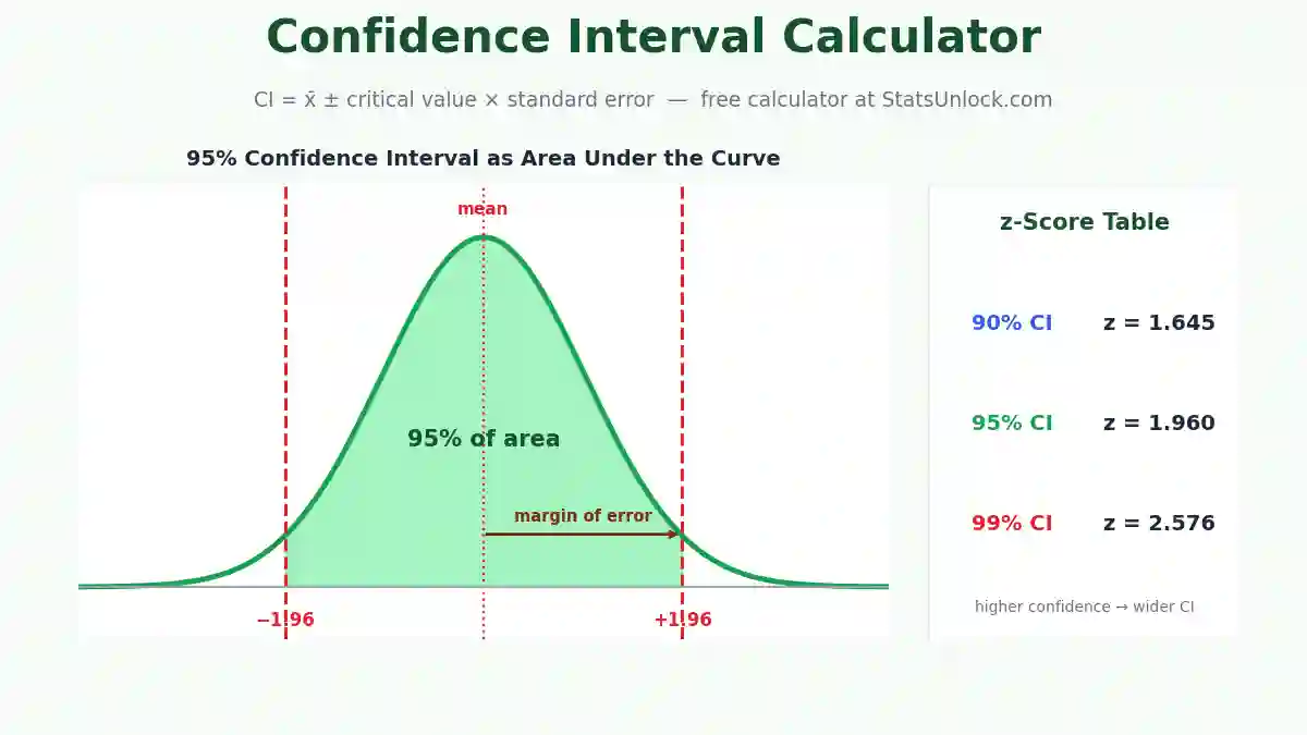
Quick answer: A confidence interval is a range of values, built from sample data, that is likely to contain the true population parameter. The formula is CI = x̄ ± critical value × standard error. For a 95% confidence interval the z-score is 1.960, for 90% it is 1.645, and for 99% it is 2.576. The margin of error is the "±" part — half the width of the interval.
🔑 Key Takeaways
- 1The confidence interval formula is estimate ± margin of error. For a mean: CI = x̄ ± t* × (s / √n). The margin of error is the critical value times the standard error.
- 2Memorize three z-scores: 1.645 for a 90% confidence interval, 1.960 for 95%, and 2.576 for 99%. Higher confidence → bigger critical value → wider interval.
- 3Use t, not z, when σ is unknown. In real research you almost never know the population standard deviation, so the t distribution with n − 1 degrees of freedom is the correct default.
- 4"95% confident" describes the method, not this one interval. If you repeated the study many times, about 95% of the intervals built this way would capture the true mean — the parameter is fixed, the intervals vary.
- 5Width shrinks with √n. To cut a margin of error in half you need four times the sample size. Width also grows with data spread (s) and with the confidence level.
- 6Margin of error vs confidence interval: the margin of error is half the interval's width. Recover it from any reported CI as (upper − lower) ÷ 2.
- 7The CI is in the same units as your data (an AP Statistics favorite): if you measure centimeters, the interval bounds are centimeters. Proportions use the binomial (Wilson or Wald) interval instead.
📥 Enter Your Data
Binomial confidence interval for a population proportion — enter the number of successes and the total number of trials:
🛠 How to Calculate a Confidence Interval with This Tool
- Enter your data. Paste comma-separated values (e.g., 52, 48, 55, 61, 47), load one of the fifteen sample datasets, or upload a CSV file and click the columns you want loaded as separate clusters. For a proportion, use the Binomial tab instead.
- Choose the level of confidence. 95% is the research standard; 90% gives a narrower interval, 99% a wider one. The level and the interval trade off directly.
- Pick the method. Keep the t interval whenever the population standard deviation is unknown (almost always). The z interval applies only when σ is known or n is very large.
- Click "Calculate Confidence Interval." The tool reports the mean, standard deviation, standard error, critical value, margin of error, and the lower and upper bounds.
- Interpret and report. Read the interval as the range of plausible values for the population mean μ, check the four charts, then copy an APA-style template from the reporting section.
📑 Confidence Interval Table: z-Scores and t-Values by Level of Confidence
These are the critical values everyone searches for. The z-score for a 95 confidence interval is 1.960; the z-value for a 90 confidence interval is 1.645; and the z-score for a 99 confidence interval is 2.576. When σ is unknown, use the t-value for your degrees of freedom (df = n − 1) instead — t is always slightly larger than z and converges to z as the sample grows.
| Confidence level | α (two tails) | z critical value | t (df = 9) | t (df = 15) | t (df = 24) | t (df = 99) |
|---|---|---|---|---|---|---|
| 80% | 0.20 | 1.282 | 1.383 | 1.341 | 1.318 | 1.290 |
| 90% | 0.10 | 1.645 | 1.833 | 1.753 | 1.711 | 1.660 |
| 95% | 0.05 | 1.960 | 2.262 | 2.131 | 2.064 | 1.984 |
| 98% | 0.02 | 2.326 | 2.821 | 2.602 | 2.492 | 2.365 |
| 99% | 0.01 | 2.576 | 3.250 | 2.947 | 2.797 | 2.626 |
How the level of confidence and confidence interval relate: the z-score marks how many standard errors you must go on each side of the mean so that the chosen percentage of the sampling distribution's area is enclosed. That is exactly what the "area under the curve" chart above shows — 95% of the area sits between −1.960 and +1.960 standard errors.
ƒ Confidence Interval Formulas Used
🔍 Confidence Interval Interpretation — In Detail
What does a 95 confidence interval mean? The precise interpretation is about the method, not any single interval: if you drew many random samples from the same population and built a 95% CI from each, about 95% of those intervals would contain the true population mean μ. The population value is fixed; it is the intervals that vary from sample to sample. The common shortcut — "we are 95% confident that μ lies between the bounds" — is acceptable in practice as long as you remember it describes confidence in the procedure.
What the interval tells you
Three readings matter. First, location: every value inside the interval is a plausible candidate for μ; values outside are implausible at the chosen level. Second, precision: a narrow interval means your estimate is precise; a wide one warns that the sample gives only a rough fix on the parameter. Third, decisions: a CI doubles as a hypothesis test — if a null value (for example, μ = 100 or a difference of 0) falls outside the 95% CI, the corresponding two-sided test rejects at α = 0.05.
Common misinterpretations to avoid
A 95% CI does not mean 95% of the data fall inside the interval — the CI describes the mean, not individual observations (that wider range is a prediction or tolerance interval). It does not mean there is a 95% probability that μ is inside this particular interval — in frequentist statistics μ either is or is not inside it. And two overlapping CIs do not automatically mean "no significant difference"; intervals can overlap up to about 25% of their combined width while the difference is still significant (Cumming & Finch, 2005).
What controls the width
The margin of error grows with the critical value (higher confidence → wider), grows with the data's spread (larger s → wider), and shrinks with the square root of the sample size (quadruple n to halve the width). This is why the 90% vs 95% vs 99% chart above shows nested intervals — same data, same mean, different guarantees. In AP Statistics terms, remember that the interval carries the same units as the variable: a CI for height in centimeters is itself a range in centimeters.
✍ How to Write Your Results in Research
Confidence intervals belong in every Results section — APA (7th edition) explicitly asks for them alongside point estimates. Report the level, both bounds in square brackets, and the units. Below are copy-ready templates; replace the bracketed values with the numbers from the results table above.
Template 1 — Single mean (t interval)
Template 2 — Reporting the margin of error
Template 3 — Comparing groups by CI
Template 4 — Binomial proportion
Reporting checklist
State the confidence level explicitly (95% CI, not just CI); give both bounds with the same decimal precision as the mean; include the units; report n; name the method if it is not the default t interval (z, Wilson, bootstrap); and prefer interpreting the interval in words over merely printing the numbers — reviewers reward it.
🔬 Example Results
Below are six worked examples using the built-in sample datasets (each n = 16, 95% t interval, t* = 2.131 at df = 15). Load any of them from the sample dropdown above to reproduce the numbers exactly.
Example 1 — Test Scores
t* = 2.131 · ME = 2.51 · 95% CI [81.18, 86.20]
With a margin of error of 2.51 points, the population mean score plausibly lies between 81.2 and 86.2. If a pass benchmark of 80 were hypothesized, it falls outside the interval — the class average is reliably above it.
Example 2 — Plant Height (cm)
t* = 2.131 · ME = 0.27 · 95% CI [24.10, 24.64]
The tiny standard deviation (0.50 cm) makes the interval only about half a centimeter wide — a very precise estimate. Consistent growing conditions show up directly as a narrow confidence interval.
Example 3 — Systolic Blood Pressure (mmHg)
t* = 2.131 · ME = 2.91 · 95% CI [122.53, 128.35]
The interval sits entirely below the 130 mmHg stage-1 hypertension threshold, so the group's mean pressure is plausibly elevated-but-not-hypertensive. Using a CI against a clinical cutoff is a common applied reading.
Example 4 — Reaction Time (ms)
t* = 2.131 · ME = 11.04 · 95% CI [203.46, 225.54]
A 22 ms wide interval reflects the large spread (SD = 20.7). To halve this margin of error you would need roughly four times the participants (n ≈ 64) — the √n rule in action.
Example 5 — Leaf Length (mm)
t* = 2.131 · ME = 2.72 · 95% CI [64.53, 69.97]
A field-botany reading: from 16 measured leaves, the species' mean leaf length plausibly lies between 64.5 and 70.0 mm. Report it as "M = 67.3 mm, 95% CI [64.5, 70.0]" and note the interval is in millimeters — the same unit as the data.
Example 6 — Same Data, Three Levels: 90% vs 95% vs 99%
90% CI [9.80, 10.06] · 95% CI [9.78, 10.08] · 99% CI [9.72, 10.14]
Same data, three levels of confidence. The 90% interval is the narrowest (z-analog 1.645), the 95% wider (1.960), and the 99% widest (2.576) — you buy extra confidence by accepting a wider range. All three intervals share the same center: the sample mean.
🧭 When to Use This Tool
Use this confidence interval calculator whenever you need to construct the confidence interval for a population mean from sample data, report a margin of error for a survey or experiment, compare group means with error bars, check whether a benchmark or hypothesized value is plausible, estimate a proportion from successes and trials with a binomial confidence interval, or teach how z-scores and confidence intervals connect. It suits researchers, students (including AP Statistics), analysts, and instructors, and works with any continuous measurement or count-based proportion.
⚠ Assumptions & Limitations
The t interval for a mean assumes the observations are independent and drawn as a random sample, and that the sampling distribution of the mean is approximately normal — guaranteed for normal data at any n, and approximately true for non-normal data once n is moderate (commonly n ≥ 30) thanks to the Central Limit Theorem. For small samples from clearly skewed or outlier-heavy data, the t interval can miscover; consider transforming the data or using a bootstrap interval. The z interval additionally assumes the population standard deviation σ is known, which is rare in practice. For proportions, the Wald interval misbehaves when n is small or p̂ is near 0 or 1 — the Wilson interval reported by this tool is the safer default (Brown, Cai & DasGupta, 2001). Finally, a confidence interval quantifies sampling uncertainty only: it cannot correct bias from non-random sampling, measurement error, or confounding.
🏁 Conclusion
A confidence interval turns a single sample estimate into an honest statement of uncertainty: estimate ± margin of error. The recipe never changes — compute the sample mean, compute the standard error (s/√n), multiply by the critical value for your level of confidence (z = 1.645 for 90%, 1.960 for 95%, 2.576 for 99%, or the slightly larger t-value when σ is unknown), and add and subtract the result from the mean.
Interpretation is where most mistakes happen, so anchor on the correct reading: the level of confidence describes the long-run success rate of the method, not the probability that this particular interval contains μ. In practice the interval earns its keep three ways — it flags every plausible value of the parameter, it exposes the precision of your study through its width, and it quietly performs a hypothesis test, rejecting any hypothesized value that falls outside it. Width is under your control: increase the sample size (quadruple n to halve the margin of error), reduce measurement noise, or accept a lower level of confidence.
This calculator gives you the full workflow: t and z intervals for the mean, Wald and Wilson intervals for a binomial proportion, the z-score table everyone searches for, four charts including the confidence-level-as-area visualization, and APA-ready reporting sentences. Run your data, read the interval in the units of your variable, and report the level, the bounds, and n — that is a complete, publication-grade confidence interval.
❓ Frequently Asked Questions
What is a confidence interval?
What does a 95 confidence interval mean?
What is the confidence interval formula?
What is the z score for a 95 confidence interval?
What is the z value for a 90 confidence interval?
What is the z score for a 99 confidence interval?
How do you calculate a 95 confidence interval by hand?
How do you find the margin of error from a confidence interval?
What is the difference between margin of error and confidence interval?
When should I use t instead of z?
How do z scores and confidence intervals relate?
Why is a 99% confidence interval wider than a 95% one?
Does a 95% CI contain 95% of the data?
How does sample size affect the confidence interval?
What is a binomial confidence interval?
Can I say there is a 95% probability the mean is in my interval?
What units is a confidence interval in (AP Stats)?
Do overlapping confidence intervals mean no significant difference?
How do I make a confidence interval narrower?
Is a confidence interval better than a p-value?
📚 References
- Neyman, J. (1937). Outline of a theory of statistical estimation based on the classical theory of probability. Philosophical Transactions of the Royal Society A, 236(767), 333–380. https://doi.org/10.1098/rsta.1937.0005
- Student (Gosset, W. S.). (1908). The probable error of a mean. Biometrika, 6(1), 1–25. https://doi.org/10.1093/biomet/6.1.1
- Cumming, G., & Finch, S. (2005). Inference by eye: Confidence intervals and how to read pictures of data. American Psychologist, 60(2), 170–180. https://doi.org/10.1037/0003-066X.60.2.170
- Brown, L. D., Cai, T. T., & DasGupta, A. (2001). Interval estimation for a binomial proportion. Statistical Science, 16(2), 101–133. https://doi.org/10.1214/ss/1009213286
- Wilson, E. B. (1927). Probable inference, the law of succession, and statistical inference. Journal of the American Statistical Association, 22(158), 209–212. https://doi.org/10.1080/01621459.1927.10502953
- Hoekstra, R., Morey, R. D., Rouder, J. N., & Wagenmakers, E.-J. (2014). Robust misinterpretation of confidence intervals. Psychonomic Bulletin & Review, 21(5), 1157–1164. https://doi.org/10.3758/s13423-013-0572-3
- Morey, R. D., Hoekstra, R., Rouder, J. N., Lee, M. D., & Wagenmakers, E.-J. (2016). The fallacy of placing confidence in confidence intervals. Psychonomic Bulletin & Review, 23(1), 103–123. https://doi.org/10.3758/s13423-015-0947-8
- Cumming, G. (2014). The new statistics: Why and how. Psychological Science, 25(1), 7–29. https://doi.org/10.1177/0956797613504966
- Gardner, M. J., & Altman, D. G. (1986). Confidence intervals rather than P values: Estimation rather than hypothesis testing. BMJ, 292(6522), 746–750. https://doi.org/10.1136/bmj.292.6522.746
- Greenland, S., Senn, S. J., Rothman, K. J., Carlin, J. B., Poole, C., Goodman, S. N., & Altman, D. G. (2016). Statistical tests, P values, confidence intervals, and power: A guide to misinterpretations. European Journal of Epidemiology, 31(4), 337–350. https://doi.org/10.1007/s10654-016-0149-3
- Efron, B., & Tibshirani, R. J. (1993). An Introduction to the Bootstrap. Chapman & Hall. https://doi.org/10.1007/978-1-4899-4541-9
- Agresti, A., & Coull, B. A. (1998). Approximate is better than "exact" for interval estimation of binomial proportions. The American Statistician, 52(2), 119–126. https://doi.org/10.1080/00031305.1998.10480550
- Newcombe, R. G. (1998). Two-sided confidence intervals for the single proportion: Comparison of seven methods. Statistics in Medicine, 17(8), 857–872. DOI link
- Belia, S., Fidler, F., Williams, J., & Cumming, G. (2005). Researchers misunderstand confidence intervals and standard error bars. Psychological Methods, 10(4), 389–396. https://doi.org/10.1037/1082-989X.10.4.389
- Altman, D. G., Machin, D., Bryant, T. N., & Gardner, M. J. (2000). Statistics with Confidence (2nd ed.). BMJ Books. Publisher page
- American Psychological Association. (2020). Publication Manual of the American Psychological Association (7th ed.). apastyle.apa.org
- Moore, D. S., McCabe, G. P., & Craig, B. A. (2021). Introduction to the Practice of Statistics (10th ed.). W. H. Freeman. Publisher page
- NIST/SEMATECH. (2012). Confidence limits for the mean. In e-Handbook of Statistical Methods. https://www.itl.nist.gov/div898/handbook/eda/section3/eda352.htm
- du Prel, J.-B., Hommel, G., Röhrig, B., & Blettner, M. (2009). Confidence interval or p-value? Deutsches Ärzteblatt International, 106(19), 335–339. https://doi.org/10.3238/arztebl.2009.0335
- Field, A. (2018). Discovering Statistics Using IBM SPSS Statistics (5th ed.). Sage. Publisher page