

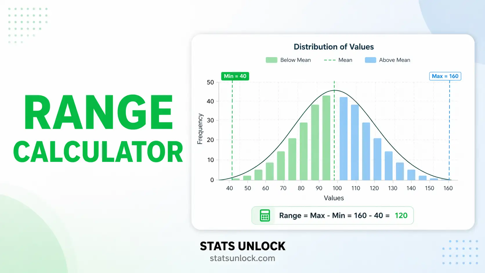

Descriptive Statistics Range Calculator
This descriptive statistics range calculator gives you every measure of spread built on the smallest and largest value. The range itself is the largest value minus the smallest. This tool gives you that plus every variant that matters: the inclusive range for whole numbers, the midrange, the interquartile range, percentile ranges, and an estimate of the standard deviation from the range using the quality-control d₂ constants.
⚡ 0. Quick Answer
range = maximum − minimumFor the values 45, 47, 48, 49, 50, 52, 54, 55, 56, 58, 61, 63 the range is 63 − 45 = 18. That is the entire calculation, and it is why the range is the first measure of spread anyone learns. Everything else on this page is a descriptive statistics range calculator built around that one subtraction: the variants, the quartile-based ranges, and the traps.
⚠ The one thing every other range calculator leaves out
The range grows as you collect more data. It is the only common measure of spread that does this. A standard deviation from 10 observations and from 1,000 observations estimate the same thing, but the range does not: with more observations you get more chances to catch an extreme value, so the range keeps climbing.
For normally distributed data the expected range is 1.13 standard deviations at n = 2, 3.08 at n = 10, 5.02 at n = 100 and 6.48 at n = 1,000. Nothing about the underlying spread changed. Only the sample size did.
The consequence: you cannot compare the range of one group against the range of another unless the two samples are the same size. Doing so is one of the most common errors in reporting, and it always makes the larger sample look more variable.
Key takeaways
- The range uses exactly two numbers and throws the rest away. With 1,000 observations, 998 of them have no influence on it whatsoever.
- It is maximally sensitive to outliers. A single mistyped value changes it completely, and the range gives you no signal that this happened.
- Use the inclusive range for counted whole numbers. Test scores from 45 to 63 span 19 possible marks, not 18. Which one you want depends on whether you are measuring a distance or counting possibilities.
- The interquartile range is the robust alternative. It describes the middle half and ignores both tails, so it is stable where the range is not.
- You can estimate a standard deviation from the range. Divide by d₂, a constant that depends on n: 2.326 at n = 5, 3.078 at n = 10. This is the basis of every X-bar and R control chart in manufacturing.
- The range rule of thumb, SD ≈ range / 4, works only around n = 15 to 30. It is badly wrong at both very small and very large sample sizes, for the same reason the range grows with n.
📚 1. What Is the Range?
1.1 The definition, and why it is the first thing anyone learns
The range is the distance from the smallest value in your data to the largest. Subtract the minimum from the maximum and you are done. No squaring, no averaging, no division, no choice of divisor.
That simplicity is its entire appeal. Anyone can compute it, anyone can check it, and it is expressed in the same units as the data. If daily temperatures ran from 4°C to 19°C, the range is 15°C, and everyone understands immediately what that means.
1.2 The five ranges people actually mean
"Range" is used loosely for several different quantities. This tool computes all of them, because which one you want depends on the question.
| Name | Formula | On the example | Use it when |
|---|---|---|---|
| Range | max − min | 63 − 45 = 18 | Measuring a distance or span on a continuous scale |
| Inclusive range | max − min + 1 | 63 − 45 + 1 = 19 | Counting how many whole values are possible |
| Midrange | (max + min) ÷ 2 | (63 + 45) ÷ 2 = 54 | A very quick centre estimate, though a fragile one |
| Interquartile range | Q3 − Q1 | 56.5 − 48.75 = 7.75 | You want a spread that outliers cannot distort |
| Semi-interquartile range | (Q3 − Q1) ÷ 2 | 7.75 ÷ 2 = 3.875 | Older texts, sometimes called the quartile deviation |
| Percentile range | P90 − P10 | 60.7 − 47.1 = 13.6 | You want to trim the extremes without going all the way to quartiles |
1.3 Why the range grows with sample size
This is the property that makes the range unlike every other measure of spread, and it is worth understanding properly.
The standard deviation estimates a fixed population quantity. Collect more data and your estimate gets more precise, but it does not systematically get bigger or smaller. The range has no such fixed target. Every new observation is another opportunity to beat the current maximum or fall below the current minimum, so the range can only ever stay the same or increase as n grows. It never decreases.
For normally distributed data the relationship is known exactly. The expected range is d₂ multiplied by the population standard deviation, where d₂ depends only on the sample size:
| Sample size | Expected range | Sample size | Expected range |
|---|---|---|---|
| n = 2 | 1.13 σ | n = 50 | 4.50 σ |
| n = 5 | 2.33 σ | n = 100 | 5.02 σ |
| n = 10 | 3.08 σ | n = 500 | 6.07 σ |
| n = 30 | 4.09 σ | n = 1,000 | 6.48 σ |
Two samples drawn from the identical population, one of 10 values and one of 1,000, will have ranges differing by more than a factor of two. Neither population is more variable than the other. This is why comparing ranges across samples of different sizes is meaningless, and why the range is unsuitable as a summary statistic in any context where sample sizes vary.
1.4 What the range does not tell you
It uses two numbers and discards everything in between. Consider two datasets that both run from 0 to 100. In the first, values are spread evenly across the whole interval. In the second, 998 values sit at 50 and one each at 0 and 100. Identical ranges, utterly different data.
The range also carries no information about the centre, the shape, or where the bulk of the data sits. It is a statement about the two most extreme observations, and extreme observations are precisely the ones most likely to be errors.
1.5 Where the range genuinely is the right choice
Despite all of that, there are situations where the range is not merely acceptable but preferred:
- Quality control with small subgroups. Taking five parts an hour and plotting the range is fast, requires no calculator, and at n = 5 the range is nearly as efficient as the standard deviation. This is why X-bar and R charts have dominated factory floors for a century.
- Specification and tolerance limits. When you need to know the worst case rather than the typical case, the extremes are the quantity of interest.
- Reporting to a non-technical audience. "Between 4 and 19 degrees" is understood instantly by everyone.
- A first sanity check. An impossible minimum or maximum reveals a data-entry error faster than any other statistic.
- Genuinely tiny samples. Below about n = 6 the range loses very little information compared with the standard deviation.
🧮 2. Set Up Your Calculation
Paste your numbers and the calculator returns every kind of range, the values that produced them, and a warning if a single extreme observation is driving the result.
📁 Or upload a CSV / Excel file
If you already know the smallest and largest values, that is all the range needs. Add the sample size and the calculator can also estimate the standard deviation.
For data already summarised into classes. The range of grouped data is an approximation, because you only know the class an observation fell into, not its actual value.
The range can estimate a standard deviation by dividing by d₂, a constant that depends on the sample size. This is how X-bar and R control charts have worked since the 1920s.
Enter several groups to compare. The calculator will warn you if the sample sizes differ, because the range cannot be compared fairly across different n.
📊 3. Results
🧠 4. Interpretation of Results, In Detail
4.1 Reading the number
The range is a distance, expressed in the same units as your data. A range of 18 marks means the best and worst results were 18 points apart. A range of 15°C means the hottest and coldest days differed by 15 degrees.
What it does not tell you is where anything sits between those two points. The range is identical whether the data cluster tightly near the middle with two stragglers at the edges, or spread evenly across the whole interval. It is a statement about two observations and nothing else.
4.2 Range or inclusive range?
Both are correct and they answer different questions. Ask yourself whether you are measuring a distance or counting possibilities.
Marks running from 45 to 63 span a distance of 18 points. But there are 19 possible whole marks in that span, because both endpoints count. This is the fencepost problem: a 10-metre fence with a post every metre needs 11 posts.
| Use the plain range when | Use the inclusive range when |
|---|---|
| Measuring a continuous quantity such as temperature, weight or time | Counting whole units such as marks, days, dice faces or people |
| Reporting how far apart the extremes are | Reporting how many distinct values are covered |
| Feeding into any statistical formula, including d₂ | Describing a span in everyday language |
| "The temperature varied by 15 degrees" | "The survey ran for 19 days" |
Statistical formulas always want the plain range. If you feed an inclusive range into a d₂ calculation you will overestimate the standard deviation, and the error is largest on small numbers.
4.3 Why the range grows with sample size, and why it matters so much
This is the most important idea on the page and it is what separates the range from every other measure of spread.
The standard deviation, the variance and the interquartile range all estimate fixed properties of the population. Collect more data and your estimates get more precise, but they do not systematically drift in one direction. The range has no fixed target to estimate. Each new observation is another chance to exceed the current maximum or fall below the current minimum, so the range can only stay the same or increase. It literally cannot decrease.
For normal data the expected range is exactly d₂ standard deviations, where d₂ depends only on n. That produces this progression:
| n | Expected range | Relative to n = 10 |
|---|---|---|
| 2 | 1.13 σ | 37% |
| 5 | 2.33 σ | 76% |
| 10 | 3.08 σ | 100% |
| 30 | 4.09 σ | 133% |
| 100 | 5.02 σ | 163% |
| 1,000 | 6.48 σ | 211% |
The fix is straightforward. Either compare groups of equal size, or compare interquartile ranges instead, or divide each range by its own d₂ constant, which is what the comparison tab does automatically.
4.4 How fragile is your range?
Because the range is built from the two most extreme observations, it is maximally exposed to exactly the values most likely to be wrong. A misplaced decimal point, a transcription slip, an instrument glitch: any of these lands at one end of the sorted data and controls the entire result.
The calculator reports what happens when you remove just one value from each end. On well-behaved data the range falls modestly. When it collapses by more than half, two observations were carrying the whole result, and you should look at them individually before reporting anything.
The ratio of the range to the interquartile range is a second useful signal. On roughly normal data it usually sits between 2 and 4, rising slowly with sample size. A ratio above about 6 means the tails are much longer than the middle, which is either genuine skew or a stray value.
4.5 The interquartile range, and when to prefer it
The interquartile range is the distance from the 25th to the 75th percentile: the span of the middle half. Because it ignores the top and bottom quarters entirely, no single extreme value can move it, and it is far more stable across different sample sizes.
Prefer the IQR whenever your data are skewed, whenever outliers are plausible, and whenever you need to compare groups. Prefer the plain range when the extremes themselves are the point, as in tolerance specifications or worst-case planning, or when your audience needs the simplest possible summary.
QUARTILE.INC, R's default type 7), Tukey's hinges, and the exclusive method (QUARTILE.EXC, R type 6) can each give a different IQR on the same data. On the twelve exam marks they give 7.75, 8.50 and 9.25 respectively. None is wrong; they answer the same question with different interpolation rules. Say which you used, and this calculator lets you switch between them.4.6 Estimating a standard deviation from the range
Divide the range by d₂ and you have an estimate of the standard deviation. This is not a rough approximation invented for convenience: d₂ is the exact expected range for a normal sample of that size, so the estimator is unbiased.
Its appeal is speed. An operator can measure five parts, subtract the smallest from the largest, and divide by 2.326 in their head. At n = 5 that estimate retains about 96% of the efficiency of a properly computed standard deviation. Walter Shewhart built control charts on exactly this trade in the 1920s, and the method survives because the efficiency loss is small where it matters and the practical gain is enormous.
Efficiency falls as subgroups grow: roughly 85% at n = 10 and below 70% by n = 20. That is precisely why control charts use small subgroups and why d₂ tables usually stop at 25. Beyond that, compute the standard deviation properly.
4.7 The range rule of thumb, and where it goes wrong
The familiar shortcut says SD ≈ range / 4. It works because d₂ happens to pass through 4 somewhere around n = 25, so for middling sample sizes the rule is close.
Outside that window it drifts badly. At n = 5, d₂ is 2.33, so dividing by 4 underestimates the standard deviation by 42%. At n = 1,000, d₂ is 6.48, so dividing by 4 overestimates it by 62%. The rule is not wrong so much as tied to a sample size nobody states when quoting it.
Use it for a quick sanity check on a moderate sample. If your computed standard deviation differs from range/4 by a factor of five, you have made an arithmetic error. For anything you intend to report, use the proper d₂ value.
4.8 Grouped data gives you a range you cannot pin down
When data arrive as a frequency table you know which class each observation fell into but not its value. That leaves two defensible answers: the distance between the outer class boundaries, which is the widest the range could possibly be, and the distance between the outer class midpoints, which is the average case.
The true range lies between them, and grouped data cannot narrow it further. The midpoint estimate is usually the more honest choice, because assuming both extreme observations sat exactly on class boundaries is an unlikely coincidence. Whichever you use, say so.
Open-ended classes make the range impossible. A top class of "60 and over" has no upper boundary, so there is no maximum and no range. Inventing a closing value is sometimes done, but that guess goes straight into the answer.
4.9 Reading the four charts
Chart 1 plots your sorted values with the minimum and maximum marked, so you can see immediately whether the extremes sit close to the rest or far out on their own. Chart 2 is the important one: it shows the expected range climbing with sample size and marks your own n on the curve. Chart 3 puts the range beside the interquartile range, the percentile range and the standard deviation, all in your original units. Chart 4 shows how fast the range shrinks as you trim values from each end, with the interquartile range drawn across for reference.
Chart 4 is the diagnostic. A steep initial drop followed by a flat stretch means one or two extreme values were doing all the work.
4.10 What to report alongside the range
Never report a range alone. At minimum give the sample size, because a range without n cannot be judged and cannot be compared with anything. Give the minimum and maximum themselves, since readers usually want to know where the span sits, not just how wide it is.
Add the interquartile range whenever there is any chance of skew or outliers. If you are comparing groups, either match the sample sizes or report the adjusted ranges, and say which you did. And if the range is the headline figure in a report, state explicitly that it is determined by two observations, so a reader knows how much weight it can bear.
✍ 5. How to Write Your Results in Research
▶ Run the analysis above to auto-fill all five examples with your results.
📌 Key conventions for this style
- Give the minimum and maximum, not just the difference. Readers want to know where the span sits.
- Always include the sample size. A range without n is uninterpretable.
- Report the interquartile range alongside whenever skew or outliers are plausible.
- Write "ranged from X to Y" rather than "the range was Z" where space allows.
📌 Key conventions for this style
- For tables, figure captions and parenthetical use.
- The convention "range 45 to 63" is clearer than "range 18" on its own.
- Keep n even when compressing.
📌 Key conventions for this style
- "From X to Y" is understood by everyone and needs no explanation.
- Avoid the word "range" as a technical term with a general audience.
- Mention the typical case as well as the extremes, or readers will assume the extremes are typical.
📌 Key conventions for this style
- State whether you used the plain or inclusive range if there is any ambiguity.
- If comparing groups, say how you handled unequal sample sizes.
- If the data were grouped, say which convention you used for the outer classes.
- Name the quartile method if you report an interquartile range.
📌 Key conventions for this style
- Reviewers increasingly ask what a dispersion figure is sensitive to.
- Say that both extremes were checked against the original records.
- Report the trimmed range or the IQR when the extremes dominate.
- Never claim one group is "more variable" from ranges alone if sample sizes differ.
∑ 6. Formulas Used
📝 7. How to Use This Calculator
- Paste your numbers into the data column. From my data opens first with one column ready. Enter values comma-separated exactly as the placeholder shows, and the calculator returns the range, the inclusive range, the midrange, the interquartile range and a trimmed percentile range all at once.
- Read the ruler diagram first. It draws the full range as a pale band with the interquartile range as a darker inner bar and every observation plotted as a dot. If the dots bunch in the middle with one stray at an end, you will see it immediately.
- Check the extremes before you trust the number. The range is built from exactly two observations, and the calculator tells you how much it falls when you remove one from each end. A drop above 50% means two values are controlling everything.
- Pick the plain or inclusive range deliberately. Plain for distances and for any statistical formula, inclusive for counting whole values. The tool shows both so the choice is visible rather than accidental.
- Load a sample dataset to see the failure modes. Nine are built in, including one where a single typo inflates the range from 18 to 585, one where every value is identical, and one showing three sample sizes drawn from the same spread.
- To compare groups, use the compare tab rather than eyeballing two ranges. It warns you when the sample sizes differ and adds a size-adjusted column, because the range grows with n and raw comparisons are misleading.
- For a frequency table, use the grouped tab. It gives both the boundary range and the midpoint range, since grouped data cannot pin the true value down to one number.
- To estimate a standard deviation, use the SD tab. Enter the range and the subgroup size and it divides by the correct d₂ constant, and optionally gives you the D₃, D₄ and A₂ factors for a control chart.
- Choose your quartile method if you care about the IQR. Linear interpolation matches Excel and R's default; Tukey hinges and the exclusive method give slightly different answers on the same data. Say which you used.
- Press Calculate Range. Nothing is computed until you do, and changing any input clears the results so you never read stale numbers.
📊 8. How to Calculate the Range in Excel
Excel has no RANGE function, which catches almost everyone the first time. You subtract MIN from MAX yourself. Below is the complete workflow in ten steps, each with a picture of what your sheet should look like.
MIN and MAX for the range itself, QUARTILE.INC for the interquartile range, PERCENTILE.INC for trimmed ranges, and LARGE and SMALL when you want the second or third most extreme value.Step 1. Put your data in one column with a header and reserve a block for the results. Twelve values sit in A2:A13; only the first eight are visible.
Step 2. MIN finds the smallest value, 45. It ignores text and blank cells.
Step 3. MAX finds the largest, 63.
Step 4. The range in a single formula. Excel has no RANGE function, which surprises people, so you subtract MIN from MAX yourself.
Step 5. The inclusive range adds 1, giving 19. Use this only when the values are whole numbers being counted, never as input to a statistical formula.
Step 6. The midrange, halfway between the two extremes. Note this is a measure of centre, not of spread, and one outlier moves it without limit.
Step 7. QUARTILE.INC uses linear interpolation and matches R's default. QUARTILE.EXC would give 48.25 instead, which is a different convention rather than an error.
Step 8. The interquartile range, 7.75. This is the robust alternative: no single extreme value can change it.
Step 9. Estimating the standard deviation. Excel has no built-in d2, so type the constant from the table in section 11 into its own cell and divide. At n = 12, d2 is 3.2585.
Step 10. The range-over-four rule gives 4.50 against the correct 5.52, an underestimate of 19%. The rule is only close for n somewhere between 15 and 30.
The complete function reference
| What you want | Excel formula | Result on the example |
|---|---|---|
| Minimum | =MIN(A2:A13) | 45 |
| Maximum | =MAX(A2:A13) | 63 |
| Range | =MAX(A2:A13)-MIN(A2:A13) | 18 |
| Inclusive range | =MAX(A2:A13)-MIN(A2:A13)+1 | 19 |
| Midrange | =(MAX(A2:A13)+MIN(A2:A13))/2 | 54 |
| First quartile | =QUARTILE.INC(A2:A13,1) | 48.75 |
| Third quartile | =QUARTILE.INC(A2:A13,3) | 56.50 |
| Interquartile range | =QUARTILE.INC(A2:A13,3)-QUARTILE.INC(A2:A13,1) | 7.75 |
| IQR, exclusive convention | =QUARTILE.EXC(A2:A13,3)-QUARTILE.EXC(A2:A13,1) | 9.25 |
| Semi-interquartile range | =(QUARTILE.INC(r,3)-QUARTILE.INC(r,1))/2 | 3.875 |
| 5th to 95th percentile range | =PERCENTILE.INC(r,0.95)-PERCENTILE.INC(r,0.05) | 15.80 |
| Second largest value | =LARGE(A2:A13,2) | 61 |
| Second smallest value | =SMALL(A2:A13,2) | 47 |
| Range after trimming one each end | =LARGE(r,2)-SMALL(r,2) | 14 |
| Range with a condition | =MAXIFS(A:A,B:B,"x")-MINIFS(A:A,B:B,"x") | Excel 2019 and later |
| SD estimated from the range | =range/d2 with d2 typed in a cell | 5.5241 at n = 12 |
| Count of values at the maximum | =COUNTIF(A2:A13,MAX(A2:A13)) | 1 |
Six mistakes that catch people out
- Looking for a RANGE function. There isn't one. In Excel, "range" means a block of cells, which is why the statistical function was never given that name.
- Forgetting the +1 when counting. If you are counting how many whole marks a span covers, you need the inclusive range. Marks from 45 to 63 cover 19 values, not 18.
- Adding the +1 to a continuous measurement. The opposite error. A temperature range of 15.3 degrees is not 16.3 degrees.
- Using QUARTILE.EXC and QUARTILE.INC interchangeably. On this data they give 9.25 and 7.75. Neither is wrong, but mixing them within one report is.
- Including the header row. Excel ignores text, so it will not error, but a numeric header becomes data and can silently become your minimum or maximum.
- Comparing ranges from ranges of different length. A range computed from 50 rows and one from 10 rows are not comparable, and no Excel formula will warn you.
QUARTILE as a legacy alias for QUARTILE.INC. MAXIFS and MINIFS are available in Sheets and in Excel 2019 or later.📈 9. How to Calculate the Range in R
R does have a range() function, but it does not return what you probably expect. This trips up almost every beginner.
range(x) returns a vector of two numbers, the minimum and the maximum, not the difference between them. range(c(45,63)) gives 45 63. To get the range as a single number you need diff(range(x)). Assigning r <- range(x) and then using r as if it were a scalar is a very common and very silent error.# Range Calculator in R (base R, no packages)
x <- c(52, 48, 55, 61, 47, 58, 50, 63, 45, 56, 54, 49)
n <- length(x)
# ---- 1. Every kind of range -------------------------------------------
range(x) # CAREFUL: returns c(min, max), NOT the range
rng <- diff(range(x)) # this is the actual range: 18
inclusive <- rng + 1 # for counted whole numbers: 19
midrange <- sum(range(x))/2 # a centre, not a spread: 54
qs <- quantile(x, c(.25, .75)) # type 7, the R default
iqr <- IQR(x) # same thing, one function
siqr <- iqr / 2
p <- quantile(x, c(.05, .95))
prng <- unname(diff(p))
# ---- 2. How much rests on two observations? ---------------------------
s <- sort(x)
trimmed <- s[n-1] - s[2] # drop one from each end
trim_pct <- (rng - trimmed) / rng * 100
# ---- 3. The d2 constant: expected range of n normals ------------------
d2 <- function(m) {
integrate(function(t) 1 - pnorm(t)^m - (1 - pnorm(t))^m,
-12, 12)$value
}
sd_actual <- sd(x)
sd_from_r <- rng / d2(n) # unbiased estimator of sigma
sd_rule <- rng / 4 # the crude rule of thumb
cat(sprintf("n = %d min = %g max = %g\n", n, min(x), max(x)))
cat(sprintf("RANGE = %g\n", rng))
cat(sprintf("inclusive range = %g\n", inclusive))
cat(sprintf("midrange = %g\n", midrange))
cat(sprintf("Q1, Q3 = %.4f, %.4f IQR = %.4f\n", qs[1], qs[2], iqr))
cat(sprintf("5th to 95th = %.4f trim one each end: %g -> %g (%.1f%% gone)\n",
prng, rng, trimmed, trim_pct))
cat(sprintf("d2(%d) = %.6f SD from range = %.6f actual SD = %.6f\n",
n, d2(n), sd_from_r, sd_actual))
cat(sprintf("range / 4 rule = %.6f\n", sd_rule))
cat("\nTHE RANGE GROWS WITH SAMPLE SIZE:\n")
for (m in c(2, 5, 10, 30, 100, 1000))
cat(sprintf(" n = %-5d expected range = %.4f sigma\n", m, d2(m)))
# ---- 4. One figure ----------------------------------------------------
plot(s, rep(0, n), pch = 19, cex = 1.6, col = "#b45309", bty = "n",
yaxt = "n", ylab = "", xlab = "value", ylim = c(-0.16, 0.16),
main = sprintf("Range and IQR n=%d, range=%g, IQR=%g", n, rng, iqr))
segments(min(x), 0, max(x), 0, lwd = 9, col = adjustcolor("#b45309", .30))
segments(qs[1], 0, qs[2], 0, lwd = 9, col = adjustcolor("#0f766e", .55))
points(s, rep(0, n), pch = 19, cex = 1.6, col = "#b45309")
segments(c(min(x), max(x)), -0.05, c(min(x), max(x)), 0.05,
lwd = 3, col = "#b45309")
text(c(min(x), max(x)), 0.08,
sprintf(c("min %g", "max %g"), c(min(x), max(x))), col = "#b45309", cex = 0.85)
segments(midrange, -0.035, midrange, 0.035, lwd = 2, col = "#0f172a")
text(midrange, -0.09, sprintf("midrange %g", midrange), cex = 0.85)
legend("topleft", bty = "n", cex = 0.85,
legend = c(sprintf("range = %g", rng), sprintf("IQR = %g", iqr)),
col = c(adjustcolor("#b45309", .5), adjustcolor("#0f766e", .7)), lwd = 9)
What the script prints
n = 12   min = 45   max = 63
RANGE           = 18
inclusive range = 19
midrange        = 54
Q1, Q3          = 48.7500, 56.5000   IQR = 7.7500
5th to 95th     = 15.8000   trim one each end: 18 -> 14 (22.2% gone)
d2(12) = 3.258455   SD from range = 5.524090   actual SD = 5.670231
range / 4 rule  = 4.500000

THE RANGE GROWS WITH SAMPLE SIZE:
  n = 2     expected range = 1.1284 sigma
  n = 5     expected range = 2.3259 sigma
  n = 10    expected range = 3.0775 sigma
  n = 30    expected range = 4.0855 sigma
  n = 100   expected range = 5.0152 sigma
  n = 1000  expected range = 6.4829 sigma
These are the same numbers the Python script produces and the same numbers the calculator at the top of this page produces.
Line-by-line explanation
- Block 1 opens with the trap deliberately visible.
range(x)on its own prints two numbers; onlydiff(range(x))gives you the range as a scalar. Note also thatIQR(x)exists as a one-word function while there is no equivalent for the plain range. - Block 2 quantifies how fragile the result is by dropping one value from each end. On clean data the fall is modest; on data with a stray value it collapses.
- Block 3 computes d₂ by numerical integration rather than looking it up, which means it works for any n rather than only the values printed in textbook tables.
- Block 4 draws the range as a wide pale bar with the interquartile range overlaid, which is the clearest way to show how much narrower the middle half is.
Useful one-liners
| Task | R | Note |
|---|---|---|
| Minimum and maximum | range(x) | returns two numbers, not one |
| The range | diff(range(x)) | this is what you usually want |
| Also the range | max(x) - min(x) | clearer to read |
| Inclusive range | diff(range(x)) + 1 | whole numbers only |
| Midrange | mean(range(x)) | neat, and it works |
| Interquartile range | IQR(x) | type 7 by default |
| IQR, other conventions | IQR(x, type = 6) | types 1 to 9 available |
| Percentile range | diff(quantile(x, c(.05,.95))) | unname() to drop the label |
| Ignore missing values | range(x, na.rm = TRUE) | otherwise NA propagates |
| Range by group | tapply(x, g, function(v) diff(range(v))) | no built-in shortcut |
| Range of every column | sapply(df, function(v) diff(range(v))) | |
| Five number summary | fivenum(x) | Tukey's version, includes both extremes |
| Everything at once | summary(x) | gives min, quartiles, median, mean, max |
| Rolling range | zoo::rollapply(x, 5, function(v) diff(range(v))) | needs the zoo package |
🐍 10. How to Calculate the Range in Python
NumPy has a dedicated function with an unhelpful name, and it is the one everybody misses. The script below was run before being published, so the output shown underneath is the real console output.
np.ptp(), short for "peak to peak". Almost nobody guesses that name, so most people write x.max() - x.min() instead, which is fine and arguably clearer. Note that ptp on an integer array can silently overflow: np.ptp(np.array([-128, 127], dtype=np.int8)) returns −1 rather than 255, because 255 does not fit in an int8. Cast to float first if your data are near the limits of their type.# Range Calculator in Python
# Range, inclusive range, midrange, IQR, percentile ranges, and the d2 estimator.
import numpy as np
import matplotlib
matplotlib.use("Agg")
import matplotlib.pyplot as plt
from scipy import stats, integrate
# ---- 1. Your data -----------------------------------------------------
x = np.array([52, 48, 55, 61, 47, 58, 50, 63, 45, 56, 54, 49], dtype=float)
n = x.size
# ---- 2. Every kind of range -------------------------------------------
lo, hi = x.min(), x.max()
rng = hi - lo # THE range: max minus min
inclusive = rng + 1 # for counted whole numbers
midrange = (hi + lo) / 2 # a centre, not a spread
q1, q3 = np.percentile(x, [25, 75]) # linear interpolation, matches Excel and R
iqr = q3 - q1
siqr = iqr / 2
p5, p95 = np.percentile(x, [5, 95])
prange = p95 - p5
# ---- 3. How much rests on two observations? ---------------------------
s = np.sort(x)
trimmed = s[-2] - s[1] # drop one from each end
trim_pct = (rng - trimmed) / rng * 100
# ---- 4. The d2 constant: expected range of n normals -------------------
def d2(m):
f = lambda t: 1 - stats.norm.cdf(t)**m - (1 - stats.norm.cdf(t))**m
return integrate.quad(f, -12, 12, limit=400)[0]
sd_actual = x.std(ddof=1)
sd_from_r = rng / d2(n) # unbiased estimator of sigma
sd_rule = rng / 4 # the crude rule of thumb
# ---- 5. Control chart constants (SPC) ---------------------------------
def PWgt(w, m):
g = lambda t: stats.norm.pdf(t)*(stats.norm.cdf(t+w) - stats.norm.cdf(t))**(m-1)
return 1 - m*integrate.quad(g, -12, 12, limit=400)[0]
def d3(m):
mu = d2(m)
e2 = integrate.quad(lambda w: 2*w*PWgt(w, m), 0, 14, limit=400)[0]
return np.sqrt(max(0.0, e2 - mu*mu))
sub = 5 # typical control chart subgroup
D3 = max(0.0, 1 - 3*d3(sub)/d2(sub))
D4 = 1 + 3*d3(sub)/d2(sub)
A2 = 3 / (d2(sub) * np.sqrt(sub))
print(f"n = {n} min = {lo:g} max = {hi:g}")
print(f"RANGE = {rng:g}")
print(f"inclusive range = {inclusive:g} (max - min + 1, for whole numbers)")
print(f"midrange = {midrange:g}")
print(f"Q1, Q3 = {q1:.4f}, {q3:.4f} IQR = {iqr:.4f} semi-IQR = {siqr:.4f}")
print(f"5th to 95th = {p5:.4f} to {p95:.4f} range = {prange:.4f}")
print(f"trim one each end: {rng:g} -> {trimmed:g} ({trim_pct:.1f}% of the range gone)")
print(f"range / IQR = {rng/iqr:.4f} (2 to 4 is typical for normal data)")
print()
print(f"d2({n}) = {d2(n):.6f}")
print(f"SD from range = {sd_from_r:.6f} actual SD = {sd_actual:.6f}"
f" error {abs(sd_from_r-sd_actual)/sd_actual*100:.1f}%")
print(f"range / 4 rule = {sd_rule:.6f}")
print()
print(f"SPC at n={sub}: d2={d2(sub):.4f} d3={d3(sub):.4f} "
f"D3={D3:.4f} D4={D4:.4f} A2={A2:.4f}")
print()
print("THE RANGE GROWS WITH SAMPLE SIZE:")
for m in (2, 5, 10, 30, 100, 1000):
print(f" n = {m:<5d} expected range = {d2(m):.4f} sigma")
# ---- 6. One figure ----------------------------------------------------
fig, ax = plt.subplots(figsize=(9, 5))
ax.scatter(s, np.zeros(n), s=90, color="#b45309", zorder=4, label="observations")
ax.hlines(0, lo, hi, color="#b45309", lw=9, alpha=.30, zorder=2,
label=f"range = {rng:g}")
ax.hlines(0, q1, q3, color="#0f766e", lw=9, alpha=.55, zorder=3,
label=f"IQR = {iqr:g}")
for v, lab in [(lo, f"min {lo:g}"), (hi, f"max {hi:g}")]:
ax.vlines(v, -0.05, 0.05, color="#b45309", lw=3, zorder=5)
ax.annotate(lab, (v, 0.07), ha="center", fontsize=9, color="#b45309")
ax.vlines(midrange, -0.035, 0.035, color="#0f172a", lw=2, zorder=5)
ax.annotate(f"midrange {midrange:g}", (midrange, -0.09), ha="center",
fontsize=9, color="#0f172a")
ax.set_ylim(-0.16, 0.16); ax.set_yticks([])
ax.set_xlabel("value")
ax.set_title(f"Range and IQR n={n}, range={rng:g}, IQR={iqr:g}")
ax.legend(frameon=False, fontsize=9, loc="upper left")
ax.spines[["top", "right", "left"]].set_visible(False)
fig.tight_layout()
fig.savefig("range.png", dpi=150)
print("saved range.png")
Actual output from running the script
n = 12   min = 45   max = 63
RANGE           = 18
inclusive range = 19   (max - min + 1, for whole numbers)
midrange        = 54
Q1, Q3          = 48.7500, 56.5000   IQR = 7.7500   semi-IQR = 3.8750
5th to 95th     = 46.1000 to 61.9000   range = 15.8000
trim one each end: 18 -> 14  (22.2% of the range gone)
range / IQR     = 2.3226   (2 to 4 is typical for normal data)

d2(12)          = 3.258455
SD from range   = 5.524090   actual SD = 5.670231   error 2.6%
range / 4 rule  = 4.500000

SPC at n=5: d2=2.3259  d3=0.8641  D3=0.0000  D4=2.1145  A2=0.5768

THE RANGE GROWS WITH SAMPLE SIZE:
  n = 2     expected range = 1.1284 sigma
  n = 5     expected range = 2.3259 sigma
  n = 10    expected range = 3.0775 sigma
  n = 30    expected range = 4.0855 sigma
  n = 100   expected range = 5.0152 sigma
  n = 1000  expected range = 6.4829 sigma
Line-by-line explanation
- Block 2 computes every variant. Note that
np.percentiledefaults to linear interpolation, which matches Excel'sQUARTILE.INCand R's type 7, so the three tools agree out of the box for once. - Block 3 measures fragility by trimming one observation from each end. On this data the range falls 22.2%, which is unremarkable. Above 50% you have a problem.
- Block 4 computes d₂ by integrating rather than looking it up, so it works for any n. The estimate of 5.5241 lands within 2.6% of the true standard deviation of 5.6702, from two numbers rather than twelve.
- Block 5 derives the control chart constants. At the standard subgroup size of 5 it produces D₄ = 2.1145 and A₂ = 0.5768, which are exactly the values printed on every SPC reference card.
- The final loop is the one worth reading twice. It prints the expected range at six sample sizes, climbing from 1.13 standard deviations at n = 2 to 6.48 at n = 1,000. Nothing about the population changed between those rows.
Useful one-liners
| Task | Python | Note |
|---|---|---|
| The range | np.ptp(x) | "peak to peak", the name nobody guesses |
| Also the range | x.max() - x.min() | clearer, and no overflow surprise |
| Minimum and maximum | x.min(), x.max() | |
| Inclusive range | np.ptp(x) + 1 | whole numbers only |
| Midrange | (x.max() + x.min()) / 2 | |
| Interquartile range | stats.iqr(x) | SciPy, linear by default |
| IQR from NumPy | np.subtract(*np.percentile(x,[75,25])) | note the reversed order |
| IQR, other conventions | stats.iqr(x, interpolation='midpoint') | several methods available |
| Percentile range | np.ptp(np.percentile(x,[5,95])) | |
| Pandas range | df['x'].max() - df['x'].min() | no built-in range method |
| Range by group | df.groupby('g')['x'].agg(lambda v: v.max()-v.min()) | |
| Range of every column | df.max() - df.min() | vectorised across columns |
| Ignore missing values | np.nanmax(x) - np.nanmin(x) | pandas skips NaN by default |
| Trimmed range | np.ptp(np.sort(x)[1:-1]) | drops one from each end |
| Rolling range | df['x'].rolling(5).apply(np.ptp) | |
| Everything at once | df.describe() | gives min and max but not the range |
📋 11. Reference Tables
11.1 The d₂ and d₃ constants, and every control chart factor built from them
This is the table that makes the range genuinely useful rather than merely simple. d₂ is the expected range of n values drawn from a normal distribution with a standard deviation of 1, so dividing your observed range by it gives an unbiased estimate of σ. d₃ is the standard deviation of the range itself, and the chart factors follow from the two.
| n | d₂ | d₃ | D₃ | D₄ | A₂ | Efficiency |
|---|---|---|---|---|---|---|
| 2 | 1.1284 | 0.8525 | 0.0000 | 3.2665 | 1.8800 | 100% |
| 3 | 1.6926 | 0.8884 | 0.0000 | 2.5746 | 1.0233 | 99% |
| 4 | 2.0588 | 0.8798 | 0.0000 | 2.2820 | 0.7286 | 98% |
| 5 | 2.3259 | 0.8641 | 0.0000 | 2.1145 | 0.5768 | 96% |
| 6 | 2.5344 | 0.8480 | 0.0000 | 2.0038 | 0.4832 | 93% |
| 7 | 2.7044 | 0.8332 | 0.0757 | 1.9243 | 0.4193 | 91% |
| 8 | 2.8472 | 0.8198 | 0.1362 | 1.8638 | 0.3725 | 89% |
| 9 | 2.9700 | 0.8078 | 0.1840 | 1.8160 | 0.3367 | 87% |
| 10 | 3.0775 | 0.7970 | 0.2230 | 1.7770 | 0.3083 | 85% |
| 11 | 3.1729 | 0.7873 | 0.2556 | 1.7444 | 0.2851 | 82% |
| 12 | 3.2585 | 0.7785 | 0.2833 | 1.7167 | 0.2658 | 82% |
| 13 | 3.3360 | 0.7704 | 0.3072 | 1.6928 | 0.2494 | 78% |
| 14 | 3.4068 | 0.7630 | 0.3281 | 1.6719 | 0.2354 | 78% |
| 15 | 3.4718 | 0.7562 | 0.3466 | 1.6534 | 0.2231 | 78% |
| 16 | 3.5320 | 0.7499 | 0.3630 | 1.6370 | 0.2123 | 72% |
| 17 | 3.5879 | 0.7440 | 0.3779 | 1.6221 | 0.2028 | 72% |
| 18 | 3.6401 | 0.7386 | 0.3913 | 1.6087 | 0.1943 | 72% |
| 19 | 3.6890 | 0.7335 | 0.4035 | 1.5965 | 0.1866 | 72% |
| 20 | 3.7349 | 0.7287 | 0.4147 | 1.5853 | 0.1796 | 72% |
| 21 | 3.7783 | 0.7242 | 0.4250 | 1.5750 | 0.1733 | 67% |
| 22 | 3.8194 | 0.7199 | 0.4345 | 1.5655 | 0.1675 | 67% |
| 23 | 3.8583 | 0.7159 | 0.4434 | 1.5566 | 0.1621 | 67% |
| 24 | 3.8953 | 0.7121 | 0.4516 | 1.5484 | 0.1572 | 67% |
| 25 | 3.9306 | 0.7084 | 0.4593 | 1.5407 | 0.1526 | 67% |
Note that D₃ is exactly zero for n below 7. That is not a rounding artefact: the lower three-sigma limit for the range falls below zero at those subgroup sizes, and a range cannot be negative, so the limit is clipped. This is why range charts with small subgroups appear to have no lower control limit.
11.2 How the range grows with sample size
The single most important table on this page. Every row describes the same underlying population; only the sample size changes.
| Sample size | Expected range | Relative to n = 10 | range / 4 as a % of the truth | Verdict |
|---|---|---|---|---|
| 2 | 1.1284 σ | 37% | 28% | under by 72% |
| 3 | 1.6926 σ | 55% | 42% | under by 58% |
| 4 | 2.0588 σ | 67% | 51% | under by 49% |
| 5 | 2.3259 σ | 76% | 58% | under by 42% |
| 6 | 2.5344 σ | 82% | 63% | under by 37% |
| 8 | 2.8472 σ | 93% | 71% | under by 29% |
| 10 | 3.0775 σ | 100% | 77% | under by 23% |
| 15 | 3.4718 σ | 113% | 87% | under by 13% |
| 20 | 3.7349 σ | 121% | 93% | under by 7% |
| 25 | 3.9306 σ | 128% | 98% | about right |
| 30 | 4.0855 σ | 133% | 102% | over by 2% |
| 50 | 4.4981 σ | 146% | 112% | over by 12% |
| 100 | 5.0152 σ | 163% | 125% | over by 25% |
| 200 | 5.4921 σ | 178% | 137% | over by 37% |
| 500 | 6.0734 σ | 197% | 152% | over by 52% |
| 1000 | 6.4829 σ | 211% | 162% | over by 62% |
11.3 The measures of spread compared
| Measure | Formula | Uses how many values? | Breakdown point | Grows with n? |
|---|---|---|---|---|
| Range | max − min | 2 | 0% | Yes, substantially |
| Interquartile range | Q3 − Q1 | about half | 25% | No |
| Semi-IQR | (Q3 − Q1) ÷ 2 | about half | 25% | No |
| 10 to 90 percentile range | P90 − P10 | about 80% | 10% | Very slightly |
| Standard deviation | √[Σ(x−x̄)²/(n−1)] | all | 0% | No |
| MAD | median of |x − median| | all | 50% | No |
| Midrange | (max + min) ÷ 2 | 2 | 0% | Not applicable, it is a centre |
Breakdown point is the fraction of the data that can be arbitrarily corrupted before the statistic becomes meaningless. The range and the midrange both have a breakdown point of zero: one bad value is enough. The MAD tolerates half the data being wrong.
11.4 Range as a multiple of the interquartile range
A useful diagnostic. For normal data this ratio rises slowly with sample size, so a value well above the expected figure points to long tails or an outlier.
| Sample size | Typical range / IQR for normal data | What a much higher value suggests |
|---|---|---|
| 10 | about 2.3 | one extreme value |
| 20 | about 2.8 | one or two extreme values |
| 50 | about 3.3 | heavy tails, or a mixture of two groups |
| 100 | about 3.7 | heavy tails or skew |
| 500 | about 4.5 | genuine long tails |
| 1,000 | about 4.8 | genuine long tails |
These are approximate because the IQR of a normal distribution is 1.349σ, so the expected ratio is simply d₂ divided by 1.349. At n = 12 that gives 3.258 / 1.349 = 2.4, against the 2.32 actually observed in the worked example.
11.5 Which range to report
| Situation | Report | Why |
|---|---|---|
| Continuous measurements, describing a span | Plain range | It is a distance |
| Counting whole values in a span | Inclusive range | Both endpoints count |
| Data are skewed | Interquartile range | The range hides which tail is long |
| Outliers are plausible | Interquartile range | The range is entirely determined by them |
| Comparing groups of different sizes | IQR, or size-adjusted range | Raw ranges are not comparable |
| Quality control with small subgroups | Plain range, plus d₂ | Fast, and nearly as efficient as the SD |
| Tolerance or specification limits | Plain range | The extremes are the point |
| Talking to a general audience | "From X to Y" | Immediately understood |
| Feeding a statistical formula | Plain range | Never the inclusive version |
11.6 The same calculation in three tools
| Task | Excel | R | Python |
|---|---|---|---|
| Minimum | MIN(r) | min(x) | x.min() |
| Maximum | MAX(r) | max(x) | x.max() |
| Range | MAX(r)-MIN(r) | diff(range(x)) | np.ptp(x) |
| Midrange | (MAX(r)+MIN(r))/2 | mean(range(x)) | (x.max()+x.min())/2 |
| IQR | QUARTILE.INC(r,3)-QUARTILE.INC(r,1) | IQR(x) | stats.iqr(x) |
| Percentile | PERCENTILE.INC(r,0.9) | quantile(x,.9) | np.percentile(x,90) |
| Named "range" function? | None exists | Yes, but returns two numbers | Yes, called ptp |
| Default quartile method | Linear (INC) | Type 7, linear | Linear |
ptp, which almost nobody finds. On the plus side, all three default to the same quartile convention, so interquartile ranges do agree across tools.💡 12. Eight Worked Examples
Every number below was computed with the calculator on this page and cross-checked against Python. Each example has its own colour and its own figure. Examples 3 and 4 are the two worth studying: one shows a single typo multiplying the range by 32, the other shows two samples from similar populations appearing to differ by a factor of nearly three purely because of their sizes.
Setup: 52, 48, 55, 61, 47, 58, 50, 63, 45, 56, 54, 49
| n | 12 |
|---|---|
| Minimum | 45 |
| Maximum | 63 |
| Range | 63 − 45 = 18 |
| Inclusive range | 18 + 1 = 19 |
| Midrange | (63 + 45) ÷ 2 = 54 |
| Q1, Q3 | 48.75, 56.50 |
| Interquartile range | 7.75 |
| Range / IQR ratio | 2.3226 |
| Mean for comparison | 53.1667 |
Reading it: The range of 18 is the distance from the lowest mark to the highest. The inclusive range of 19 is the number of possible whole marks in that span, and which you want depends on whether you are measuring a distance or counting possibilities. Notice how much narrower the interquartile range is: the middle half of the class sits within 7.75 marks, less than half the full spread. The range-to-IQR ratio of 2.32 is unremarkable for twelve observations, so no single mark is stretching the result.
Setup: The same marks, 45 to 63. How wide is the span, and how many marks does it cover?
| Question A | How far apart are the best and worst marks? |
|---|---|
| Answer A | 18 marks apart |
| Question B | How many different whole marks are possible in that span? |
| Answer B | 19 possible marks |
| Why they differ | both endpoints are counted in B, only the gap in A |
| The classic analogy | a 10 m fence with posts every metre needs 11 posts |
| Use plain for | temperature, weight, time, any statistical formula |
| Use inclusive for | marks, days, dice faces, anything counted |
Reading it: Neither answer is wrong, and confusing them is the fencepost error. Days 1 to 7 of a study span a distance of 6 days but cover 7 days of observation. The rule that matters in practice: any statistical formula, including the d2 estimator on this page, wants the plain range. Feeding it an inclusive range inflates the result, and the error is proportionally largest on small numbers, where the extra 1 is a big share of the total.
Setup: 52, 48, 55, 61, 47, 58, 50, 63, 45, 56, 54, 49, 630
| n | 13 |
|---|---|
| Minimum | 45 |
| Maximum | 630 (should be 63) |
| Range | 585 |
| Range without the typo | 18 |
| Range after trimming one at each end | 16 |
| Drop from trimming | 97.3% |
| Interquartile range | 9.00 |
| Range / IQR ratio | 65.0 |
| What the IQR did | barely moved, from 7.75 to 9.00 |
Reading it: A single misplaced digit multiplies the range by 32. Removing just one value from each end cuts it by 97.3%, which is the clearest possible signal that the statistic is describing one observation rather than a dataset. Note what the interquartile range did: it moved from 7.75 to 9.00 and no further, because the middle half of the data is untouched by anything happening in the tails. This is the entire case for reporting the IQR alongside, and the range-to-IQR ratio of 65 is a red flag no reader could miss.
Setup: Two samples drawn from populations with very similar spread: one of 5 values, one of 50.
| Small sample | 43, 45, 49, 56, 61 (n = 5) |
|---|---|
| Large sample | a 50-value set with almost the same spread |
| Small sample SD | 7.5631 |
| Large sample SD | 7.5593 |
| SD ratio | 1.00, the spread is genuinely identical |
| Small sample range | 18 |
| Large sample range | 28 |
| Range ratio | 1.56, from sample size alone |
| d₂ at n = 5 and n = 50 | 2.3259 and 4.4981, a ratio of 1.93 |
| Size-adjusted ranges | 7.739 and 6.225 |
Reading it: These two samples have essentially identical spread: their standard deviations are 7.5631 and 7.5593, a ratio of 1.00. Yet their ranges are 18 and 28, a ratio of 1.56. That entire difference comes from sample size, because every extra observation is another chance to set a new extreme and the range can only grow with n. It never shrinks. The d₂ constants predict a ratio of 1.93 purely from the sizes, and dividing each range by its own d₂ brings the two figures to 7.74 and 6.23, far closer than 18 against 28 suggested. The adjustment slightly overshoots here because the range of a single five-value sample is itself very variable, which is a second reason to distrust ranges from tiny samples. The practical rule stands: comparing raw ranges across unequal sample sizes always makes the larger sample look more variable, and it is the most common misuse of this statistic.
Setup: Five parts measured off a production line: 10.02, 9.98, 10.05, 9.96, 10.01 mm.
| Subgroup size n | 5 |
|---|---|
| Minimum | 9.96 |
| Maximum | 10.05 |
| Range | 0.09 |
| d₂ for n = 5 | 2.3259 |
| Estimated SD | 0.038694 |
| Actual SD | 0.035071 |
| Estimation error | 10.3% |
| Range / 4 rule | 0.0225, which is 42% too low |
| D₄ for n = 5 | 2.1145, so the range chart UCL is 0.1903 |
| A₂ for n = 5 | 0.5768 |
Reading it: An operator subtracts two numbers and divides by 2.326. The estimate of 0.0387 lands 10% above the standard deviation of 0.0351 computed properly from all five values, which is about the accuracy you should expect from a single subgroup of this size. At n = 5 the range estimator retains about 96% of the efficiency of the full calculation, which is why Shewhart built control charts around it in the 1920s and why they still work this way. Note that the range-over-four rule gives 0.0225 here, 42% too low, because d2 at n = 5 is 2.326 rather than 4. The rule of thumb silently assumes a sample size nobody ever states.
Setup: The same twelve exam marks, with the interquartile range computed three ways.
| Linear interpolation Q1, Q3 | 48.75, 56.50 |
|---|---|
| Linear IQR | 7.75 |
| Tukey hinges Q1, Q3 | 48.50, 57.00 |
| Tukey IQR | 8.50 |
| Exclusive Q1, Q3 | 48.25, 57.50 |
| Exclusive IQR | 9.25 |
| Spread between methods | 1.50 marks |
| The plain range | 18 under every method |
| Excel default | QUARTILE.INC, the linear method |
| R default | type 7, also the linear method |
Reading it: The interquartile range is 7.75, 8.50 or 9.25 depending on which convention you use, a spread of 1.5 marks on identical data. None is wrong; they interpolate differently between the two observations straddling each quartile. The plain range is 18 under all three, because minima and maxima need no interpolation, which is one genuine advantage of the range over the IQR: it is completely unambiguous. If an IQR you compute disagrees with someone elses, check the method before you check the arithmetic.
Setup: Ages in five classes: 0 to 10 (3 people), 10 to 20 (7), 20 to 30 (12), 30 to 40 (6), 40 to 50 (2).
| Total frequency | 30 |
|---|---|
| Classes | 5 |
| Class width | 10 |
| Lowest boundary | 0 |
| Highest boundary | 50 |
| Boundary range | 50 |
| Lowest midpoint | 5 |
| Highest midpoint | 45 |
| Midpoint range | 40 |
| Uncertainty | 10 years |
| If the top class were open-ended | no range could be computed at all |
Reading it: Grouping records which class each person fell into and discards their actual age. The youngest person is somewhere between 0 and 10, the oldest somewhere between 40 and 50, so the true range is anywhere from 30 to 50. The boundary method assumes both sat exactly on the outer edges, which is the most extreme case; the midpoint method assumes the average case and gives 40. The midpoint estimate is usually the more honest one, but say which you used, because a reader cannot tell from the number. And if the top class had been 40 and over, there would be no maximum and no range at all.
Setup: 22, 25, 27, 28, 31, 33, 34, 36, 39, 42, 48, 55, 71, 96, 180 (thousands)
| n | 15 |
|---|---|
| Minimum | 22 |
| Maximum | 180 |
| Range | 158 |
| Interquartile range | 22.00 |
| Range / IQR ratio | 7.2 |
| 10th to 90th percentile range | 60.20 |
| Median | 36.00 |
| Mean | 51.13 |
| Skewness | 2.62, strongly right-skewed |
| Range after trimming one each end | 71 |
Reading it: The range says incomes span 158 thousand. The interquartile range says the middle half of households sit within 22 thousand of each other. Both are true and they describe completely different realities. The range treats both ends alike, so it entirely conceals the fact that this distribution has a short left tail and a very long right one. The range-to-IQR ratio of 7.2 is far above the 2 to 4 expected for symmetric data, which is the diagnostic. For skewed data like this, report the median with the interquartile range, and quote the range only if the extremes are themselves the point.
📋 13. Data Collection Protocol
The range is built from the two most extreme observations, which are exactly the values most likely to be errors. That single fact should shape how you collect and check data whenever a range is going to be reported.
- Verify both extremes against the original record. Not the spreadsheet, the original. A misplaced decimal or a transposed digit lands at one end of the sorted data and controls the entire result, as Example 3 shows.
- Fix the sample size in advance if you intend to compare groups. The range grows with n, so unequal sample sizes make any comparison meaningless. Equal n is the only clean solution.
- Record the sample size alongside every range you report. A range without n cannot be interpreted or compared with anything.
- Use one measurement protocol throughout. Mixing instruments or conditions widens the extremes with measurement noise that has nothing to do with the quantity you are studying.
- Watch for values at a detection or instrument limit. Readings recorded as "below detection" or capped at a maximum truncate the tails and understate the range, sometimes dramatically.
- Never record missing data as zero. A zero becomes your minimum and the range balloons. Blanks are excluded; zeros are not.
- Record raw values at full resolution. Rounding compresses the extremes and shrinks the range, and coarse rounding can make several values tie at the minimum or maximum.
- Decide plain or inclusive before you start. It depends on whether you are measuring a distance or counting whole values, and the decision belongs in the protocol rather than being made at the reporting stage.
- Avoid open-ended categories if a range will be needed. A top class of "60 and over" makes the maximum unknowable and the range uncomputable.
- Plot the data before summarising it. A dot plot takes seconds and immediately reveals whether the extremes sit close to the rest or far out on their own.
- Report the interquartile range alongside whenever skew or outliers are plausible, which is most of the time.
- For quality control, keep subgroups small and consistent. Four or five is standard, because that is where the range is nearly as efficient as the standard deviation and the d₂ constant stays stable.
🎯 14. When to Use the Range, and When Not To
Use the range when
- The extremes are the point. Tolerance limits, worst-case planning, safety margins and specification checks all care about the boundaries rather than the typical case.
- You are running quality control with small subgroups. At n = 4 or 5 the range is roughly as informative as the standard deviation and vastly faster to compute by hand.
- Your audience is non-technical. "Between 4 and 19 degrees" needs no explanation to anyone.
- You are sanity-checking new data. An impossible minimum or maximum exposes a data-entry error faster than any other statistic.
- The sample is genuinely tiny. Below about n = 6 you lose very little by using the range instead of the standard deviation.
- You need something completely unambiguous. Unlike quartiles, the range has no competing conventions: every tool agrees on the minimum and maximum.
Do not rely on the range when
- You are comparing groups of different sizes. This is the big one. The range grows with n, so the comparison is contaminated before you start.
- Outliers are plausible and unverified. One bad value controls the result completely, and the range gives you no warning.
- The data are skewed. The range treats both tails alike and hides the fact that one is far longer than the other.
- You have a large sample. With 1,000 observations the range is determined by two of them and ignores 998. That is an enormous waste of information.
- The data are ordinal. The distance between rank 1 and rank 5 is not a meaningful quantity.
- You need a measure that supports further analysis. Almost nothing in inferential statistics is built on the range, whereas the standard deviation is the foundation of most of it.
- Values may be censored or capped. A truncated tail makes the range meaningless rather than merely imprecise.
What to use instead
| Situation | Better choice | Why |
|---|---|---|
| Comparing groups of unequal size | Interquartile range or standard deviation | Neither grows systematically with n |
| Outliers present | Interquartile range | Ignores the tails entirely |
| Skewed data | Median with quartiles | Shows which tail is long |
| Large samples | Standard deviation | Uses every observation |
| You want a robust spread in original units | 1.4826 × MAD | Breakdown point of 50% |
| Ordinal data | Frequencies or the range of ranks | Arithmetic on ranks is not meaningful |
| Quality control with larger subgroups | S charts rather than R charts | The range loses efficiency above about n = 10 |
| Reporting uncertainty in an estimate | Confidence interval | The range describes data, not estimates |
| Reference intervals in medicine | 2.5th to 97.5th percentile range | Stable, and excludes the extreme 5% |
🔧 15. Troubleshooting
| Symptom | Cause | Fix |
|---|---|---|
R's range(x) gave two numbers | That function returns the minimum and maximum, not their difference | Use diff(range(x)) or max(x)-min(x) |
| You cannot find a RANGE function in Excel | There isn't one; "range" means a block of cells | =MAX(r)-MIN(r) |
| You cannot find a range function in NumPy | It is called np.ptp, for "peak to peak" | Or just x.max()-x.min() |
np.ptp returned a negative number | Integer overflow on a small dtype | Cast to float first, or use max minus min |
| Your answer is one more than expected | You used the inclusive range | Drop the +1 for distances and for any formula |
| Your answer is one less than expected | You needed the inclusive range | Add 1 when counting whole values in a span |
| The range is enormous | One value in the wrong unit, or a typo adding a digit | Sort the data and inspect both extremes |
| The range is zero | Every value is identical | Correct, but check for rounding or copy errors |
| Group A looks far more variable than group B | Group A probably has more observations | Compare IQRs, or divide each range by its d₂ |
| Your IQR does not match a colleague's | Different quartile convention | Linear, Tukey and exclusive give 7.75, 8.50 and 9.25 on the same data |
| The plain range matches but the IQR does not | Same cause. Minima and maxima need no interpolation | Agree on a quartile method |
| SD estimated from the range is badly wrong | You divided by 4 instead of d₂ | At n = 5 divide by 2.326, not 4 |
| Grouped range does not match the raw range | Grouping is an approximation | Expected. Report which convention you used |
| You cannot compute a range at all | An open-ended class such as "60 and over" | No maximum exists. Report the closed classes only |
| Excel included your header row | A numeric header is treated as data | Start the range at the first data row |
| Missing values were treated as zero | Blanks and zeros behave differently | Leave missing cells genuinely blank |
⚖ 16. Assumptions and Limitations
What the range assumes
The subtraction itself assumes nothing at all. Everything below is about whether the resulting number means what you want it to mean.
| Assumption | How much it matters | What happens if it fails | How to check |
|---|---|---|---|
| Both extremes are genuine | Critical | The range describes a typo rather than your data | Verify the two values against the original record |
| Sample sizes match, when comparing | Critical | The larger sample always appears more variable | Compare n before comparing ranges |
| Interval or ratio scale | High | The distance between ordinal codes is not a quantity | Inspect what the numbers represent |
| No censoring or capping | High | Truncated tails make the range meaningless, not just imprecise | Look for values piled up at a limit |
| Roughly symmetric, for interpretation | Moderate | The range hides which tail is long | Compare the mean with the median |
| Normality, for the d₂ estimator only | Moderate | The SD estimate drifts on skewed data | Only relevant when using d₂ |
| Classes closed, for grouped data | Critical for that mode | An open-ended class makes the range uncomputable | Check the first and last classes |
| Correct variant chosen | Moderate | Off by exactly 1, which is proportionally large on small numbers | Distance or count? |
Limitations worth stating in a write-up
- It uses two observations and discards the rest. With 1,000 values, 998 have no influence. No other common statistic throws away so much.
- It grows with sample size. This is unique among measures of spread and it makes cross-group comparison invalid unless n matches.
- Its breakdown point is zero. A single corrupted value destroys it, and the statistic itself gives no signal that this happened.
- It says nothing about shape or centre. Data clustered tightly with two stragglers and data spread evenly give the identical range.
- It has no sampling theory worth using. There is no standard confidence interval for a range in routine practice, and almost no inferential procedure is built on it.
- The range-over-four rule is tied to an unstated sample size. It returns 58% of the correct standard deviation at n = 5 and 162% at n = 1,000.
- Grouped ranges are ambiguous by construction. Two defensible answers exist and the data cannot distinguish between them.
- The midrange is even more fragile than the range. As a measure of centre it has a breakdown point of zero, which is why the mean and median exist.
🏁 17. Conclusion
The range is the largest value minus the smallest. It is the first measure of spread anyone learns, it needs no formula, and it is expressed in the same units as the data. For describing a span to a general audience, for checking new data for impossible values, and for quality control with small subgroups, it remains genuinely the right choice.
Three variants are worth keeping straight. The plain range is a distance and is what every statistical formula expects. The inclusive range adds one and counts how many whole values a span covers, which is the right answer when you are counting marks or days rather than measuring a gap. The interquartile range describes the middle half and is the robust alternative to reach for whenever the extremes cannot be trusted.
Two properties of the range cause almost all of the trouble. The first is that it rests on exactly two observations, which are precisely the values most likely to be typos. Example 3 on this page shows a single misplaced digit multiplying the range by 32, with 97% of the result disappearing when one value is trimmed from each end. The interquartile range, over the same data, barely moved. That contrast is the entire argument for reporting both.
The second property is the one almost nobody mentions and it is the reason this page exists. The range grows with sample size. It is the only common measure of spread that does, because every additional observation is another chance to set a new extreme and the range can never decrease. For normal data the expected range climbs from 1.13 standard deviations at n = 2 to 3.08 at n = 10, 5.02 at n = 100 and 6.48 at n = 1,000, with the population unchanged throughout. Example 4 shows two samples whose standard deviations agree to two decimal places producing ranges that differ by more than half. Comparing raw ranges across groups of different sizes is therefore not a rough approximation, it is a systematic error that always makes the larger sample look more variable.
That same relationship, read the other way, is what makes the range useful in manufacturing. Divide by the d₂ constant for your subgroup size and you have an unbiased estimate of the standard deviation from two numbers and a division. At n = 5 that estimate retains roughly 96% of the efficiency of the full calculation, which is why Shewhart built control charts on it in the 1920s and why D₃, D₄ and A₂ still appear on every SPC reference card. Note that the familiar range-over-four shortcut is a special case of this that quietly assumes n is somewhere around 25; at n = 5 it returns 58% of the correct answer.
So: report the range with its sample size, always. Give the minimum and maximum rather than just the difference, because readers want to know where the span sits. Verify both extremes before you publish. Add the interquartile range whenever skew or outliers are plausible. And never, under any circumstances, compare the range of one group against the range of another unless the two samples are the same size.
❓ 18. Frequently Asked Questions
What is the range in statistics?
How do you calculate the range?
=MAX(range)-MIN(range), in R it is diff(range(x)) and in Python it is np.ptp(x) or simply x.max()-x.min(). No sorting is strictly necessary, though sorting makes the extremes easy to eyeball.What is the difference between the range and the inclusive range?
Why does the range increase with sample size?
Can I compare the range of two groups?
Why is Excel's range function missing?
=MAX(A2:A13)-MIN(A2:A13). There is no hidden function to find.Why does R's range() function give two numbers?
range(x) returns a vector containing the minimum and the maximum, not the difference between them. To get the range as a single number use diff(range(x)) or max(x)-min(x). Assigning r <- range(x) and then treating r as a scalar is the most common R error on this topic, and it fails silently rather than raising an error.What is np.ptp in Python?
x.max() - x.min() instead, which is clearer and avoids one real hazard: on small integer types np.ptp can overflow silently. np.ptp(np.array([-128,127], dtype=np.int8)) returns −1 rather than 255, because 255 does not fit in an int8.What is the midrange?
Is the range affected by outliers?
What is the difference between the range and the interquartile range?
How do I estimate the standard deviation from the range?
Why is the range rule of thumb SD equals range over 4?
What are d₂, D₃, D₄ and A₂?
Why is D₃ zero for small subgroups?
Can the range be zero or negative?
How do I find the range of grouped data?
Is the range a good measure of spread?
What is a percentile range?
Why does my interquartile range not match someone else's?
QUARTILE.INC, R's type 7), Tukey's hinges and the exclusive method (QUARTILE.EXC, R type 6) give 7.75, 8.50 and 9.25 on the same twelve values. None is wrong; they interpolate differently between the observations straddling each quartile. The plain range, by contrast, is identical under every method, because minima and maxima need no interpolation.🔖 19. Cite This Tool
🔗 20. Related Calculators
📖 21. Glossary
| Term | Meaning |
|---|---|
| Range | Maximum minus minimum. A distance, in the units of the data. |
| Inclusive range | Maximum minus minimum plus one. Counts how many whole values a span covers. |
| Midrange | The average of the minimum and maximum. A measure of centre, not spread. |
| Interquartile range (IQR) | Q3 minus Q1, the spread of the middle half. |
| Semi-interquartile range | Half the IQR. Also called the quartile deviation. |
| Percentile range | A trimmed range, such as the 10th to 90th percentile. |
| Quartile | A value cutting the data at 25%, 50% or 75%. |
| Tukey hinges | One convention for quartiles, using the medians of the two halves. |
| Breakdown point | The fraction of data that can be corrupted before a statistic fails. Zero for the range. |
| Outlier | A value far from the rest. It determines the range entirely. |
| d₂ | The expected range of n normal values with a standard deviation of 1. |
| d₃ | The standard deviation of the range itself. |
| D₃, D₄ | Multipliers giving the control limits for a range chart. |
| A₂ | The multiplier giving X-bar chart limits from the average range. |
| R chart | A control chart plotting subgroup ranges over time. |
| X-bar chart | A control chart plotting subgroup means, usually paired with an R chart. |
| Subgroup | A small sample taken at one time for quality control, typically four or five items. |
| Efficiency | How much information an estimator extracts relative to the best available one. |
| Statistical process control | Monitoring a process using control charts, where the range is still widely used. |
| Range rule of thumb | SD approximately equals range divided by 4. Only accurate near n = 25. |
| Grouped data | A frequency table. Ranges from it are approximate. |
| Class boundary | The stated edge of a class interval. |
| Class midpoint | The centre of a class interval. |
| Open-ended class | A class such as "60 and over", which makes the range uncomputable. |
| Fencepost error | Confusing a count of items with the gaps between them. The source of the plus-one confusion. |
| Censored data | Values recorded only as above or below a limit, which truncates the range. |
| Trimmed range | The range after removing a fixed number of values from each end. |
📚 22. References
- Shewhart, W. A. (1931). Economic Control of Quality of Manufactured Product. Van Nostrand. archive.org
- Tippett, L. H. C. (1925). On the extreme individuals and the range of samples taken from a normal population. Biometrika, 17(3-4), 364-387. doi.org/10.1093/biomet/17.3-4.364
- Pearson, E. S. (1932). The percentage limits for the distribution of range in samples from a normal population. Biometrika, 24(3-4), 404-417. doi.org/10.1093/biomet/24.3-4.404
- Hartley, H. O. (1942). The range in random samples. Biometrika, 32(3-4), 334-348. doi.org/10.1093/biomet/32.3-4.334
- David, H. A., & Nagaraja, H. N. (2003). Order Statistics (3rd ed.). Wiley. doi.org/10.1002/0471722162
- Duncan, A. J. (1986). Quality Control and Industrial Statistics (5th ed.). Irwin. archive.org
- Montgomery, D. C. (2020). Introduction to Statistical Quality Control (8th ed.). Wiley. wiley.com
- Wheeler, D. J., & Chambers, D. S. (2010). Understanding Statistical Process Control (3rd ed.). SPC Press. spcpress.com
- American Society for Quality (2019). ASQ Control Chart Constants. asq.org
- Tukey, J. W. (1977). Exploratory Data Analysis. Addison-Wesley. archive.org
- Hyndman, R. J., & Fan, Y. (1996). Sample quantiles in statistical packages. The American Statistician, 50(4), 361-365. doi.org/10.1080/00031305.1996.10473566
- Moore, D. S., McCabe, G. P., & Craig, B. A. (2021). Introduction to the Practice of Statistics (10th ed.). W. H. Freeman. macmillanlearning.com
- Wan, X., Wang, W., Liu, J., & Tong, T. (2014). Estimating the sample mean and standard deviation from the sample size, median, range and interquartile range. BMC Medical Research Methodology, 14, 135. doi.org/10.1186/1471-2288-14-135
- Hozo, S. P., Djulbegovic, B., & Hozo, I. (2005). Estimating the mean and variance from the median, range, and the size of a sample. BMC Medical Research Methodology, 5, 13. doi.org/10.1186/1471-2288-5-13
- Gumbel, E. J. (1958). Statistics of Extremes. Columbia University Press. archive.org
- Harter, H. L. (1960). Tables of range and studentized range. Annals of Mathematical Statistics, 31(4), 1122-1147. doi.org/10.1214/aoms/1177705684
- Huber, P. J., & Ronchetti, E. M. (2009). Robust Statistics (2nd ed.). Wiley. doi.org/10.1002/9780470434697
- Harris, C. R., et al. (2020). Array programming with NumPy. Nature, 585, 357-362. doi.org/10.1038/s41586-020-2649-2
- Virtanen, P., et al. (2020). SciPy 1.0: Fundamental algorithms for scientific computing in Python. Nature Methods, 17, 261-272. doi.org/10.1038/s41592-019-0686-2
- R Core Team (2024). R: A Language and Environment for Statistical Computing. R Foundation for Statistical Computing. r-project.org