

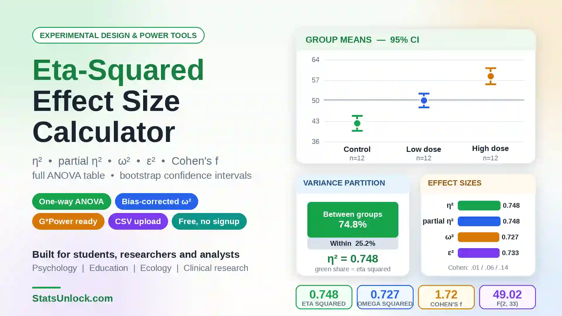

Eta-Squared Effect Size Calculator
Paste your groups as comma-separated values and get eta squared, partial eta squared, omega squared, epsilon squared and Cohen's f, together with the full one-way ANOVA table, bootstrap confidence intervals and four publication-ready plots.
Key takeaways
- Eta squared (η²) = SSbetween / SStotal - the share of total variance explained by group membership.
- Cohen's rough benchmarks: 0.01 small, 0.06 medium, 0.14 large - but field context beats any fixed cutoff.
- In a one-way ANOVA, eta squared and partial eta squared are identical. They diverge only with two or more factors.
- η² is biased upward; its expected value under a true null is about (k−1)/(N−1). Report ω² alongside it, especially for small samples.
- Cohen's f = √(η² / (1 − η²)) is the value G*Power asks for in a power analysis.
1. Set Up Your Data
Use + on any column to insert another group beside it, and × to remove it. You need at least two groups; a one-way ANOVA usually has three or more.
Click the columns that should each become a cluster - selected columns will be loaded as separate clusters.
2. Results
Group summary
One-way ANOVA table
Effect size measures
Visualisations
3. Interpretation of Results - In Detail
3.1 What eta squared actually measures
Eta squared answers one question: of all the variation in your outcome, what share can be attributed to which group an observation belongs to? If η² = 0.25, then a quarter of the total spread in your data is explained by the grouping factor and three quarters is unexplained - individual differences, measurement error, and everything you did not control for. It is a proportion, so it is bounded between 0 and 1 and is unit-free, which is exactly why it travels well across studies that measured different things on different scales.
The arithmetic is a partition. The total sum of squares measures how far every observation sits from the grand mean. That total splits cleanly into a between-groups piece, driven by how far each group mean sits from the grand mean, and a within-groups piece, driven by how far observations sit from their own group mean. Eta squared is simply the first piece divided by the whole. Nothing is thrown away and nothing overlaps, which is why the variance-partition plot in section 2 is a genuine, exact picture and not an approximation.
3.2 Reading the magnitude
Cohen proposed 0.01, 0.06 and 0.14 as small, medium and large. Those numbers have become conventions, and this tool labels your result against them, but treat them as a starting point rather than a verdict. Cohen himself described them as arbitrary and intended for situations where no better yardstick exists.
- η² < 0.01 - negligible. Group membership tells you almost nothing about the outcome.
- 0.01 to 0.06 - small. Common and often meaningful in psychology, education and epidemiology, where outcomes have many causes.
- 0.06 to 0.14 - medium. Visible in a plot, useful in practice.
- > 0.14 - large. Standard in controlled laboratory work, agronomy and dose-response experiments, where the manipulation is strong and the noise is low.
A field-appropriate benchmark beats a universal one every time. A η² of 0.03 for a classroom intervention delivered at national scale may matter enormously; a η² of 0.30 in a tightly controlled bench experiment may be unremarkable. Say what your value means for the decision at hand, not just which Cohen bucket it lands in.
3.3 Eta squared versus partial eta squared
This is the single most misreported pair of numbers in the applied literature. In a one-way ANOVA they are mathematically identical, because there is only one factor and nothing else to remove from the denominator. This calculator prints both so you can see that for yourself.
They diverge as soon as you add a second factor. Eta squared keeps the full total sum of squares in the denominator, so all the effects in a model sum to at most 1. Partial eta squared removes the other effects, using SSeffect / (SSeffect + SSerror), so each effect is judged against only its own error term. Partial values are therefore always at least as large, they do not sum to 1, and they grow as you add more controlled factors to the design. Comparing a partial eta squared from a complex factorial against a plain eta squared from a one-way study is an apples-to-oranges comparison that quietly inflates the apparent effect. If you report partial values, label them unambiguously as partial.
3.4 Why eta squared is biased, and what to do about it
Eta squared is a ratio of sample sums of squares, and sampling noise always pushes group means slightly apart even when the population means are identical. The consequence is that η² is never zero and is systematically too large. Its expected value when the null hypothesis is exactly true is approximately (k−1)/(N−1). With three groups and fifteen observations in total, that expectation is about 0.14 - precisely the value convention calls "large". At small sample sizes, a large eta squared can be produced by nothing whatsoever.
Two corrections address this, and the tool computes both:
- Omega squared (ω²) subtracts the expected noise using the within-groups mean square. It is the best estimator of the population effect and is what most methodologists now recommend as the primary report. It can come out negative, which is not an error - it is the estimator telling you the observed effect is no larger than chance.
- Epsilon squared (ε²) applies a similar correction with the total sum of squares in the denominator. It sits between η² and ω² and is the effect size R's
rstatixand several ANOVA packages report by default.
The gap between η² and ω² is a direct readout of how much bias your design carries. If they are close, your sample is doing its job. If η² is much larger, treat your point estimate with suspicion and lean on the confidence interval.
3.5 Reading the confidence interval
A point estimate without an interval is half a result. This tool computes a bootstrap percentile interval: it resamples within each group with replacement, recomputes η² thousands of times, and reports the empirical percentiles. That approach makes no assumption about the shape of the sampling distribution, which matters because the distribution of η² is skewed and bounded at zero.
Two things to check. First, width: an η² of 0.25 with an interval of 0.10 to 0.42 is a very different claim from the same 0.25 with an interval of 0.01 to 0.61. Second, the lower bound: because η² cannot be negative, the interval rarely includes zero even for a null effect, so do not use "the interval excludes zero" as a significance test. Use the F test for that and the interval for precision. Note also that a bootstrap interval for η² is generally narrower and slightly optimistic compared with an exact noncentral-F interval; treat it as a good practical guide rather than an exact coverage guarantee.
3.6 Decision guide - which effect size should you report?
| Your situation | Report this | Also give | Why |
|---|---|---|---|
| One-way ANOVA, n ≥ 20 per group | η² | ω², 95% CI | Bias is modest and η² is what readers expect |
| One-way ANOVA, small samples | ω² | η² for comparability | η² is materially inflated below about n = 20 |
| Factorial or repeated-measures ANOVA | partial η² | generalised η² | Label it clearly; never compare it to a one-way η² |
| Two groups only | Cohen's d | η² = r² | Readers in most fields expect d for a two-group contrast |
| Planning a future study | Cohen's f | ω² as the input | G*Power takes f; using an inflated η² underpowers your next study |
| Meta-analysis input | ω² or f | F, df, group n | Pooling biased estimates biases the pooled result |
| Non-normal data, Kruskal-Wallis | ε² (rank-based) | η²H | The classical η² assumes the ANOVA model |
3.7 Common mistakes this calculator prevents
- Calling a one-way partial eta squared "different". It is not. If a paper reports both as different values for a single-factor design, something is wrong.
- Reporting η² from a pilot study as if it were unbiased. Use ω² and expect the real effect to be smaller.
- Feeding η² into a power analysis. G*Power wants Cohen's f, and it should be derived from a bias-corrected estimate.
- Treating a large η² as evidence that every group differs. The omnibus effect can be driven by one deviant group; always plot the means and run post-hoc tests.
- Ignoring unequal variances. If Levene's test flags heteroscedasticity, the F test and the classical η² both become unreliable; switch to Welch's ANOVA.
- Confusing variance explained with importance. A small η² on a life-or-death outcome can matter far more than a large one on a trivial measure.
4. How to Report Eta-Squared in a Research Paper
4.1 Methods section
4.2 Results section - sentence templates
Significant, large effect:
Significant, moderate effect:
Non-significant result - do not call it "no effect":
APA 7th style note. Report η² to two decimals with no leading zero (η² = .26), give F with both degrees of freedom in parentheses, and place the effect size after the p-value in the same statistical string.
4.3 Table and figure conventions
- Give the full ANOVA table (source, SS, df, MS, F, p) in supplementary material so readers can recompute your effect size.
- Report group n, mean and standard deviation for every group - effect sizes cannot be checked without them.
- Use η² = .26, not 0.26 or 26%, in APA-style text.
- State explicitly whether a reported value is eta squared, partial eta squared or generalised eta squared.
- Plot group means with confidence intervals, not bare bar charts - readers need to see the overlap.
- If you ran post-hoc comparisons, give an effect size for each contrast as well as the omnibus one.
4.4 Discussion section
Three things reviewers will ask about. Is the effect size interpreted against a field-appropriate benchmark rather than Cohen's labels alone? Is the bias in eta squared acknowledged if the sample is small? And is the omnibus effect broken down, so readers know whether all groups differ or just one? Address all three before submission and the review will go faster.
5. Formulas Used
SSbetween = Σ nj (x̄j − x̄)²
SSwithin = Σ Σ (xij − x̄j)²
partial η² = SSbetween / (SSbetween + SSwithin)
MSbetween = SSbetween / df1 MSwithin = SSwithin / df2
F = MSbetween / MSwithin
ε² = [SSbetween − df1 × MSwithin] / SStotal
η² = f² / (1 + f²)
d = 2f (two equal-sized groups)
η² from a published test: η² = (F × df1) / (F × df1 + df2)
compute η²(b)
CI = [ percentileα/2, percentile1−α/2 ] of the B values
6. How to Use This Calculator
- Load a sample from the dropdown to see the tool work, or clear it and paste your own data.
- One column per group. Paste comma-separated values into each column; the counts and means update as you type.
- Name your groups. The names are editable and flow into every table and plot.
- Add or remove groups with the + and × buttons on each column header. Two is the minimum.
- Or upload a CSV and click the columns you want; each selected column becomes its own group.
- Choose the confidence level and bootstrap size, then press Calculate.
- Read the results: KPI cards, the plain-English summary, group summary, the ANOVA table, the effect-size table and four plots.
- Download the .txt for your analysis log so your numbers stay reproducible.
7. Reference Tables
7.1 Interpreting the magnitude of eta squared
| η² | Variance explained | Cohen's label | Cohen's f | Typical context |
|---|---|---|---|---|
| 0.01 | 1% | Small | 0.10 | Large-scale social or education interventions |
| 0.03 | 3% | Small to medium | 0.18 | Epidemiology, survey research |
| 0.06 | 6% | Medium | 0.25 | Applied psychology, clinical outcomes |
| 0.10 | 10% | Medium to large | 0.33 | Well-controlled field experiments |
| 0.14 | 14% | Large | 0.40 | Cohen's threshold for a large effect |
| 0.25 | 25% | Very large | 0.58 | Strong laboratory manipulations |
| 0.50 | 50% | Extremely large | 1.00 | Dose-response, agronomy, calibration studies |
7.2 Expected eta squared under a true null (the bias table)
This is the value you would get on average from data with no real effect at all, approximately (k−1)/(N−1). Compare your result against the relevant row before you celebrate.
| Groups (k) | n per group | Total N | Expected η² under H₀ | Cohen label of that noise |
|---|---|---|---|---|
| 3 | 5 | 15 | 0.143 | Large |
| 3 | 10 | 30 | 0.069 | Medium |
| 3 | 20 | 60 | 0.034 | Small to medium |
| 3 | 50 | 150 | 0.013 | Small |
| 4 | 10 | 40 | 0.077 | Medium |
| 4 | 30 | 120 | 0.025 | Small |
| 5 | 10 | 50 | 0.082 | Medium |
| 5 | 40 | 200 | 0.020 | Small |
7.3 Converting between effect size measures
| From | To | Formula | Note |
|---|---|---|---|
| η² | Cohen's f | f = √(η²/(1−η²)) | The G*Power input |
| Cohen's f | η² | η² = f²/(1+f²) | Reverse of the above |
| η² (k = 2) | Cohen's d | d = 2√(η²/(1−η²)) | Equal group sizes |
| F, df | η² | η² = F·df₁/(F·df₁+df₂) | Recover from a published paper |
| η² | r (correlation) | r = √η² | Exact when k = 2 |
| η² | ω² | needs SS and MSwithin | Not recoverable from η² alone |
7.4 Approximate sample size for a given effect (80% power, α = .05)
| Target η² | Cohen's f | k = 3, n per group | k = 4, n per group | k = 5, n per group |
|---|---|---|---|---|
| 0.01 | 0.10 | ~322 | ~274 | ~240 |
| 0.02 | 0.14 | ~160 | ~136 | ~120 |
| 0.06 | 0.25 | ~52 | ~45 | ~39 |
| 0.10 | 0.33 | ~30 | ~26 | ~23 |
| 0.14 | 0.40 | ~21 | ~18 | ~16 |
| 0.25 | 0.58 | ~11 | ~10 | ~9 |
Indicative values from the noncentral F distribution; confirm with G*Power or an exact power calculator before committing to a design.
7.5 What each effect size measure is for
| Measure | Range | Bias | Best use |
|---|---|---|---|
| Eta squared (η²) | 0 to 1 | Upward | Descriptive share of variance; the default reader expectation |
| Partial eta squared | 0 to 1 | Upward, larger | Factorial and repeated-measures designs only |
| Omega squared (ω²) | can be < 0 | Nearly unbiased | Population estimate; small samples; meta-analysis |
| Epsilon squared (ε²) | can be < 0 | Nearly unbiased | R default in several packages; rank-based ANOVA |
| Cohen's f | 0 to ∞ | Follows η² | Power analysis input |
| Generalised η² | 0 to 1 | Upward | Comparing across mixed within/between designs |
8. Example Results
Ten fully worked cases covering the situations you are most likely to meet: large and null effects, tiny samples where the bias bites, unbalanced groups, a two-group design, a dose-response gradient, and applications from agronomy, education, ecology, clinical research, environmental monitoring and psychology. Each card shows the group summary, the ANOVA table, every effect size, a figure, what the numbers mean, and a sentence you can adapt for your manuscript.
Fertiliser and plant height
Large effect - treatment explains most of the variance
A randomised glasshouse trial grew 36 seedlings under three fertiliser regimes and measured final height in centimetres after eight weeks. Groups are balanced and variances look similar.
| Group | n | Mean (cm) | SD |
|---|---|---|---|
| Control | 12 | 42.58 | 3.74 |
| Low dose | 12 | 48.19 | 2.79 |
| High dose | 12 | 56.42 | 2.96 |
| Source | SS | df | MS |
|---|---|---|---|
| Between | 1163.33 | 2 | 581.67 |
| Within | 335.83 | 33 | 10.18 |
| Total | 1499.16 | 35 | - |
| ε² / magnitude | 0.762 | Large effect | |
Eta-squared here is large by any convention: the treatment accounts for a substantial majority of the total variation in height. Two things are worth noticing. First, with balanced groups and healthy sample sizes, eta-squared and omega-squared are close, which tells you the upward bias in eta-squared is small. Second, a large eta-squared does not by itself tell you which doses differ - that requires post-hoc comparisons. Report the effect size for the omnibus test, then follow with Tukey contrasts.
"Fertiliser and plant height differed significantly across the 3 groups, F(2, 33) = 57.16, p < .001, η² = .78, ω² = .76. Group membership accounted for approximately 78% of the total variance, a large effect by Cohen's conventions."
Teaching method and exam score
Moderate effect - the typical size in education research
Sixty students were randomly assigned to four instructional formats and sat the same end-of-term examination scored out of 100.
| Group | n | Mean (points) | SD |
|---|---|---|---|
| Lecture | 15 | 61.67 | 4.89 |
| Flipped | 15 | 71.29 | 8.92 |
| Blended | 15 | 66.57 | 9.64 |
| Online | 15 | 59.99 | 6.69 |
| Source | SS | df | MS |
|---|---|---|---|
| Between | 1171.77 | 3 | 390.59 |
| Within | 3378.97 | 56 | 60.34 |
| Total | 4550.74 | 59 | - |
| ε² / magnitude | 0.218 | Large effect | |
This is the size of effect most educational interventions actually produce, and it is worth internalising as a benchmark. Cohen's thresholds (0.01 small, 0.06 medium, 0.14 large) were never meant as universal law, and in education a value near 0.10 is a genuinely useful intervention. The overlap between group distributions remains large, so individual students in the weakest format still outperform many in the strongest - an important caveat to state when the result is used for policy.
"Teaching method and exam score differed significantly across the 4 groups, F(3, 56) = 6.47, p < .001, η² = .26, ω² = .21. Group membership accounted for approximately 26% of the total variance, a large effect by Cohen's conventions."
No real difference between groups
Small eta-squared that is still not zero - and why
Three samples of twenty observations were drawn from the same underlying population, so the true effect is exactly zero.
| Group | n | Mean (units) | SD |
|---|---|---|---|
| Group A | 20 | 47.76 | 8.67 |
| Group B | 20 | 51.98 | 6.99 |
| Group C | 20 | 48.95 | 7.81 |
| Source | SS | df | MS |
|---|---|---|---|
| Between | 189.49 | 2 | 94.75 |
| Within | 3516.47 | 57 | 61.69 |
| Total | 3705.96 | 59 | - |
| ε² / magnitude | 0.018 | Small effect | |
The critical lesson: eta-squared is never zero even when the null hypothesis is exactly true. Because it is a ratio of sums of squares, sampling noise always assigns some variance to the group factor. Its expected value under the null is roughly (k−1)/(N−1), which here is about 0.034. Omega-squared corrects for this and can go negative, which is your signal that the observed effect is no larger than chance. If you report a small eta-squared without omega-squared alongside it, readers cannot tell a weak real effect from pure noise.
"No real difference between groups did not differ significantly across the 3 groups, F(2, 57) = 1.54, p = .224, η² = .05, ω² = .02. The small omega squared indicates that the observed spread between group means is consistent with sampling variation."
Camera-trap activity across habitats
Moderate effect in a field survey with real-world noise
Fifty-six camera stations were distributed across four habitat types and detection rates standardised to detections per 100 trap-nights.
| Group | n | Mean (detections / 100 nights) | SD |
|---|---|---|---|
| Forest | 14 | 19.29 | 5.63 |
| Edge | 14 | 26.32 | 3.92 |
| Grassland | 14 | 15.56 | 4.85 |
| Wetland | 14 | 20.51 | 4.96 |
| Source | SS | df | MS |
|---|---|---|---|
| Between | 836.78 | 3 | 278.93 |
| Within | 1238.09 | 52 | 23.81 |
| Total | 2074.87 | 55 | - |
| ε² / magnitude | 0.369 | Large effect | |
Habitat explains a moderate share of the variation in activity, which is a realistic result for field ecology where weather, moon phase and individual ranging behaviour all add unexplained variance. Before you interpret this causally, check the assumption that stations are independent - stations within the same habitat patch usually are not, which inflates the apparent effect. A mixed model with patch as a random effect is the proper follow-up, and its variance components will give you a more honest partition than a one-way ANOVA can.
"Camera-trap activity across habitats differed significantly across the 4 groups, F(3, 52) = 11.71, p < .001, η² = .40, ω² = .36. Group membership accounted for approximately 40% of the total variance, a large effect by Cohen's conventions."
Drug dose and blood pressure reduction
Dose-response gradient produces a very large effect
Sixty-four hypertensive patients were randomised to placebo or one of three doses; the outcome is the reduction in systolic blood pressure at twelve weeks.
| Group | n | Mean (mmHg) | SD |
|---|---|---|---|
| Placebo | 16 | 1.11 | 5.04 |
| 10 mg | 16 | 8.37 | 5.48 |
| 20 mg | 16 | 12.51 | 4.64 |
| 40 mg | 16 | 19.64 | 3.97 |
| Source | SS | df | MS |
|---|---|---|---|
| Between | 2884.69 | 3 | 961.56 |
| Within | 1391.13 | 60 | 23.19 |
| Total | 4275.81 | 63 | - |
| ε² / magnitude | 0.658 | Large effect | |
A monotone dose-response ordering concentrates the between-group sum of squares and drives eta-squared high. When your groups are ordered like this, the omnibus ANOVA is arguably the wrong test: a linear trend contrast has more power and answers the scientific question directly. Report eta-squared for the omnibus effect, then the trend contrast with its own effect size. Also translate back to the original scale - a 17 mmHg mean difference between placebo and the top dose is what a clinician actually needs.
"Drug dose and blood pressure reduction differed significantly across the 4 groups, F(3, 60) = 41.47, p < .001, η² = .67, ω² = .65. Group membership accounted for approximately 67% of the total variance, a large effect by Cohen's conventions."
Five observations per group
Eta-squared is badly upward-biased at tiny sample sizes
A pilot study measured only five units at each of three sites.
| Group | n | Mean (units) | SD |
|---|---|---|---|
| Site 1 | 5 | 26.84 | 1.92 |
| Site 2 | 5 | 40.04 | 3.11 |
| Site 3 | 5 | 31.52 | 5.96 |
| Source | SS | df | MS |
|---|---|---|---|
| Between | 447.89 | 2 | 223.94 |
| Within | 195.25 | 12 | 16.27 |
| Total | 643.14 | 14 | - |
| ε² / magnitude | 0.646 | Large effect | |
With N = 15 and k = 3, the expected eta-squared under a true null is about 0.14 - the exact value Cohen calls 'large'. In other words, at this sample size a 'large' eta-squared is what you get from nothing at all. The gap between eta-squared and omega-squared here is the bias made visible. Never report eta-squared alone from a pilot study, never use it to justify a follow-up sample size without correcting it, and treat any confidence interval as very wide.
"Five observations per group differed significantly across the 3 groups, F(2, 12) = 13.76, p < .001, η² = .70, ω² = .63. Group membership accounted for approximately 70% of the total variance, a large effect by Cohen's conventions."
Unequal group sizes
Eta-squared handles unbalanced designs without adjustment
An observational survey collected 8 rural, 20 suburban and 14 urban respondents, so group sizes are markedly unequal.
| Group | n | Mean (score) | SD |
|---|---|---|---|
| Rural | 8 | 54.24 | 8.33 |
| Suburban | 20 | 61.74 | 7.85 |
| Urban | 14 | 66.58 | 7.41 |
| Source | SS | df | MS |
|---|---|---|---|
| Between | 776.61 | 2 | 388.30 |
| Within | 2371.01 | 39 | 60.80 |
| Total | 3147.62 | 41 | - |
| ε² / magnitude | 0.208 | Large effect | |
Sums of squares are weighted by group size automatically, so eta-squared is well defined for unbalanced data and needs no correction. The real risk in unbalanced designs is elsewhere: the F test becomes sensitive to unequal variances when the group sizes differ. Check Levene's test, and if variances differ, use Welch's ANOVA and report an effect size derived from it rather than the classical eta-squared.
"Unequal group sizes differed significantly across the 3 groups, F(2, 39) = 6.39, p = .004, η² = .25, ω² = .20. Group membership accounted for approximately 25% of the total variance, a large effect by Cohen's conventions."
Two groups only
Eta-squared equals r-squared, and converts to Cohen's d
A two-arm trial with eighteen participants per arm - the simplest possible one-way design.
| Group | n | Mean (score) | SD |
|---|---|---|---|
| Treated | 18 | 69.78 | 11.29 |
| Control | 18 | 58.76 | 10.97 |
| Source | SS | df | MS |
|---|---|---|---|
| Between | 1093.40 | 1 | 1093.40 |
| Within | 4212.73 | 34 | 123.90 |
| Total | 5306.13 | 35 | - |
| ε² / magnitude | 0.183 | Large effect | |
With two groups, eta-squared is exactly the squared point-biserial correlation between group membership and the outcome, and it converts directly to Cohen's d via d = 2√(η²/(1−η²)) for equal group sizes. Reviewers in psychology and medicine usually expect d for a two-group comparison, so convert before you submit. The tool prints Cohen's f, which is simply √(η²/(1−η²)) - half of d in the balanced two-group case.
"Two groups only differed significantly across the 2 groups, F(1, 34) = 8.82, p = .005, η² = .21, ω² = .18. Group membership accounted for approximately 21% of the total variance, a large effect by Cohen's conventions."
Dissolved oxygen along a river
Very large effect driven by one degraded reach
Dissolved oxygen was measured at ten dates across five river reaches, one of which sits immediately below a wastewater outfall.
| Group | n | Mean (mg/L) | SD |
|---|---|---|---|
| Upstream | 10 | 8.98 | 0.84 |
| Mid 1 | 10 | 8.47 | 0.64 |
| Mid 2 | 10 | 8.15 | 0.73 |
| Outfall | 10 | 5.27 | 0.54 |
| Downstream | 10 | 7.39 | 0.59 |
| Source | SS | df | MS |
|---|---|---|---|
| Between | 84.17 | 4 | 21.04 |
| Within | 20.59 | 45 | 0.46 |
| Total | 104.76 | 49 | - |
| ε² / magnitude | 0.786 | Large effect | |
The very large eta-squared is real but almost entirely attributable to a single reach. This is the classic case where an omnibus effect size hides its own structure: four of the five reaches are similar, and one is not. Always plot the group means before you write the sentence. Reporting 'reach explained 78% of the variance' without adding 'driven by the outfall reach' would be technically true and practically misleading.
"Dissolved oxygen along a river differed significantly across the 5 groups, F(4, 45) = 46.00, p < .001, η² = .80, ω² = .78. Group membership accounted for approximately 80% of the total variance, a large effect by Cohen's conventions."
Sleep deprivation and reaction time
Small-to-moderate effect with heavy distribution overlap
Fifty-four participants were assigned to one of three sleep durations and completed a simple reaction-time task the following morning.
| Group | n | Mean (ms) | SD |
|---|---|---|---|
| 8 hours | 18 | 415.89 | 49.60 |
| 6 hours | 18 | 427.22 | 45.50 |
| 4 hours | 18 | 477.11 | 45.40 |
| Source | SS | df | MS |
|---|---|---|---|
| Between | 38193.04 | 2 | 19096.52 |
| Within | 112056.67 | 51 | 2197.19 |
| Total | 150249.70 | 53 | - |
| ε² / magnitude | 0.225 | Large effect | |
The group means differ in the expected direction and the effect reaches conventional significance, but eta-squared shows that sleep condition explains only a modest share of the variance - individual differences in baseline reaction speed dominate. This is the norm in cognitive psychology and it is why within-subject designs are preferred: they remove between-person variance from the denominator and raise the effect size for the same underlying phenomenon. Note that partial eta-squared from a repeated-measures version of this study would be substantially larger and is not comparable to the value shown here.
"Sleep deprivation and reaction time differed significantly across the 3 groups, F(2, 51) = 8.69, p < .001, η² = .25, ω² = .22. Group membership accounted for approximately 25% of the total variance, a large effect by Cohen's conventions."
9. When to Use This Calculator
Use it when
- You have run or are writing up a one-way ANOVA and need an effect size to accompany the F test.
- You have two or more independent groups measured on a continuous outcome.
- A reviewer has asked you to add effect sizes to a manuscript that reported only p-values.
- You need Cohen's f as the input to a power analysis in G*Power for a planned study.
- You want to check whether an eta squared reported in a published paper is consistent with its F and degrees of freedom.
- You are teaching or learning variance partitioning and want to see SSbetween, SSwithin and the resulting ratio side by side.
- You suspect your sample is too small for eta squared to be trustworthy and want omega squared for comparison.
Do not use it when
- Your design has more than one factor. A two-way or factorial ANOVA needs partial or generalised eta squared computed from that model, not from a one-way partition.
- Your measurements are repeated on the same subjects. Within-subject designs remove between-person variance and require a repeated-measures model; the value here would be wrong.
- Your outcome is categorical. Use Cramér's V or an odds ratio instead.
- Your groups are ordered and you want a trend. A linear contrast is more powerful and more informative than an omnibus effect size.
- Variances differ markedly between groups. Run Welch's ANOVA and report an effect size derived from it; the classical partition assumes homogeneity.
- Your data are strongly non-normal or heavily tied. Use Kruskal-Wallis with a rank-based epsilon squared.
- Observations are clustered or nested (sites, classrooms, litters, camera blocks). Use a mixed model and read the variance components.
- You only have summary statistics. If you have F and its degrees of freedom, use the conversion in section 7.3 rather than this data-entry tool.
10. Assumptions and Limitations
- Independence. Every observation belongs to exactly one group and is independent of the others. This is the assumption that clustered field data most often break.
- Normality of residuals. The F test assumes approximately normal residuals within each group; it is fairly robust with balanced groups and n above about 15.
- Homogeneity of variance. Group variances are assumed equal. Check Levene's test, especially when group sizes differ.
- Continuous outcome measured on an interval or ratio scale.
- Eta squared is descriptive, not inferential. It describes your sample; omega squared estimates the population.
- Upward bias. η² is inflated in small samples and cannot be zero. Always read it against the section 7.2 bias table.
- Sensitive to design, not just to the phenomenon. Restricting the range of your groups, adding controlled factors, or using a within-subject design all change the effect size for the same underlying effect. This is why effect sizes are only comparable across studies with comparable designs.
- Outliers. Because sums of squares involve squared deviations, a single extreme value can move η² substantially. Inspect plot 3 before trusting the number.
- The bootstrap interval is a percentile interval and tends to be slightly narrow; an exact noncentral-F interval is preferable when precision matters.
- No causal claim. Variance explained is association. Only the design, not the statistic, can license a causal interpretation.
11. Conclusion
Eta squared exists because a p-value answers the wrong question. Significance tells you whether an effect is distinguishable from zero given your sample size, and with a large enough sample almost anything is. What a reader actually needs to know is how much of the variation in the outcome your grouping factor accounts for, and that is what eta squared reports: a single, unit-free proportion between zero and one that can be compared across studies measuring completely different quantities. Reporting it is now expected by the APA, by CONSORT, and by most journals in psychology, education, ecology and the health sciences, and reporting it alongside the F test costs you one extra line.
The most consequential decision is which member of the family to report. In a one-way design, eta squared and partial eta squared are the same number, and knowing that immediately protects you from the most common misreading in the applied literature, where a partial value from a factorial design is compared against a plain value from a simpler one. As soon as a second factor enters the model the two separate, partial values become systematically larger, and comparability across studies quietly disappears unless every author labels their measure precisely. Say which one you computed, every time.
The second decision is whether to trust your point estimate. Eta squared is a ratio of sample sums of squares, so sampling noise alone guarantees a non-zero value, and the smaller your sample the larger that floor becomes. With three groups of five, chance alone delivers an eta squared of roughly 0.14, exactly the number convention calls large. Omega squared removes that expected noise and is the better estimate of what is true in the population, which is why methodologists increasingly ask for it as the primary report. The distance between your eta squared and your omega squared is a free diagnostic: when they nearly coincide, your design is adequate; when they diverge, your point estimate is flattering you.
Finally, resist letting Cohen's three thresholds do your thinking. They were offered as rough guidance in the absence of anything better, and they are a poor substitute for a benchmark drawn from your own literature. An effect that explains three per cent of the variance in a national education programme may change more lives than one explaining thirty per cent in a bench experiment, and an omnibus effect size will happily conceal the fact that a single deviant group is producing all of it. Report the effect size, report its bias-corrected companion, report an interval, plot the group means, and then tell the reader what the number means for the decision they have to make. Done that way, eta squared stops being a box to tick and becomes the most informative sentence in your results section.
12. Frequently Asked Questions
What is eta squared in simple terms?
It is the proportion of the total variation in your outcome that is explained by which group an observation belongs to. An eta squared of 0.20 means 20% of the spread in your data is attributable to the grouping factor and 80% is not.
What is a good eta squared value?
Cohen's benchmarks are 0.01 small, 0.06 medium and 0.14 large, but these are rough. Compare your value against typical effects in your own field rather than against a universal cutoff.
Is eta squared the same as partial eta squared?
In a one-way ANOVA, yes - exactly the same number. They differ only when the model contains more than one factor, where partial eta squared removes the other factors from the denominator and is therefore larger.
Is eta squared the same as R squared?
For a one-way ANOVA they are the same quantity: the share of variance explained by the model. R squared is the regression name for it.
Why is my eta squared not zero when there is no effect?
Because it is a ratio of sample sums of squares, random noise always pushes group means slightly apart. Its expected value under a true null is about (k−1)/(N−1). Use omega squared, which corrects for this.
Can omega squared be negative?
Yes, and it is not an error. A negative omega squared means the observed between-group variance is smaller than what sampling noise alone would produce. Report it as approximately zero and note the negative value.
How do I convert eta squared to Cohen's d?
For two equal-sized groups, d = 2√(η²/(1−η²)). With more than two groups there is no single d, because d describes a pair.
How do I get eta squared from a published paper?
If the paper reports F and both degrees of freedom, use η² = (F × df₁) / (F × df₁ + df₂). That recovers the effect size exactly for a one-way design.
Which effect size should I put into G*Power?
Cohen's f. This tool prints it. Derive it from omega squared rather than eta squared if you are planning a new study, or you will underpower it.
Do I need equal group sizes?
No. Sums of squares are weighted by group size automatically, so eta squared is valid for unbalanced data. Unequal sizes do make the F test more sensitive to unequal variances, so check that assumption.
What is the minimum sample size?
There is no hard rule, but below about ten per group the bias in eta squared is severe. Twenty or more per group keeps the bias small; see the table in section 7.2.
What if my data are not normally distributed?
The F test is reasonably robust with balanced groups. For serious departures, run a Kruskal-Wallis test and report a rank-based epsilon squared instead.
What if my group variances are very different?
Use Welch's ANOVA. The classical partition and the eta squared derived from it both assume homogeneity of variance.
Can I use this for repeated-measures data?
No. Repeated measurements on the same participants violate independence and require a within-subjects model; partial eta squared from that model is the correct statistic.
Does a large eta squared mean every group differs?
No. An omnibus effect can be produced by a single deviant group. Plot the means and run post-hoc comparisons such as Tukey's HSD.
How many decimal places should I report?
Two, in APA style, with no leading zero: η² = .26. Give F to two decimals and exact p-values to three.
What is the difference between epsilon squared and omega squared?
Both correct the upward bias. Epsilon squared divides by the total sum of squares; omega squared adds the within-groups mean square to the denominator. Omega squared is very slightly more conservative; the two are usually close.
Why is the bootstrap interval not symmetric?
Because the sampling distribution of eta squared is skewed and bounded at zero. An asymmetric interval is the correct result, not a bug.
Does this work on a phone?
Yes. The layout, all tables, the input columns and the four plots reflow to a single column on small screens.
Is my data uploaded anywhere?
No. Every calculation, the bootstrap and all four plots run entirely in your browser. Nothing is transmitted.
13. Cite This Tool
Free to use and free to reference. If this calculator helped with an analysis, a citation or a link is appreciated.
StatsUnlock. (2026). Eta-Squared Effect Size Calculator [Interactive statistical tool]. https://statsunlock.com/eta-squared-effect-size-calculator/
@misc{statsunlock_etasq_2026,
  title  = {Eta-Squared Effect Size Calculator},
  author = {{StatsUnlock}},
  year   = {2026},
  note   = {Interactive statistical tool},
  url    = {https://statsunlock.com/eta-squared-effect-size-calculator/}
}
Effect sizes for the one-way analysis of variance were calculated using the StatsUnlock Eta-Squared Effect Size Calculator (statsunlock.com). Eta squared was computed as the between-groups sum of squares divided by the total sum of squares, with omega squared reported alongside it to correct for upward bias, and 95% confidence intervals obtained by within-group bootstrap resampling with 2,000 replicates.
14. Related Tools
Part of the StatsUnlock experimental design and power toolkit - all free, no signup, and they work together.
Feed the Cohen's f from this page straight in to get the sample size per group you need for 80% or 90% power.
Open the tool →The effect size to use when your outcome is binary rather than continuous, with CIs, NNT and forest plots.
Open the tool →Work out the visitors per variant you need before launching a two-arm experiment.
Open the tool →See alpha, beta and power as areas under two curves and how effect size drives them.
Open the tool →15. References
- Cohen J. (1988). Statistical Power Analysis for the Behavioral Sciences, 2nd ed. Routledge. doi:10.4324/9780203771587
- Cohen J. (1992). A power primer. Psychological Bulletin, 112(1), 155–159. doi:10.1037/0033-2909.112.1.155
- Lakens D. (2013). Calculating and reporting effect sizes to facilitate cumulative science. Frontiers in Psychology, 4, 863. doi:10.3389/fpsyg.2013.00863
- Olejnik S, Algina J. (2003). Generalized eta and omega squared statistics. Psychological Methods, 8(4), 434–447. doi:10.1037/1082-989X.8.4.434
- Olejnik S, Algina J. (2000). Measures of effect size for comparative studies. Contemporary Educational Psychology, 25(3), 241–286. doi:10.1006/ceps.2000.1040
- Levine TR, Hullett CR. (2002). Eta squared, partial eta squared, and misreporting of effect size. Human Communication Research, 28(4), 612–625. doi:10.1111/j.1468-2958.2002.tb00828.x
- Richardson JTE. (2011). Eta squared and partial eta squared as measures of effect size. Educational Research Review, 6(2), 135–147. doi:10.1016/j.edurev.2010.12.001
- Keselman HJ. (1975). A Monte Carlo investigation of three estimates of treatment magnitude. Canadian Psychological Review, 16(1), 44–48. doi:10.1037/h0081789
- Hays WL. (1963). Statistics for Psychologists. Holt, Rinehart and Winston. WorldCat entry
- Kelley TL. (1935). An unbiased correlation ratio measure. PNAS, 21(9), 554–559. doi:10.1073/pnas.21.9.554
- Steiger JH. (2004). Beyond the F test: effect size confidence intervals. Psychological Methods, 9(2), 164–182. doi:10.1037/1082-989X.9.2.164
- Smithson M. (2001). Correct confidence intervals for various regression effect sizes. Educational and Psychological Measurement, 61(4), 605–632. doi:10.1177/00131640121971392
- Fritz CO, Morris PE, Richler JJ. (2012). Effect size estimates: current use, calculations, and interpretation. Journal of Experimental Psychology: General, 141(1), 2–18. doi:10.1037/a0024338
- Efron B, Tibshirani RJ. (1993). An Introduction to the Bootstrap. Chapman & Hall. doi:10.1201/9780429246593
- Welch BL. (1951). On the comparison of several mean values. Biometrika, 38(3–4), 330–336. doi:10.1093/biomet/38.3-4.330
- Levene H. (1960). Robust tests for equality of variances. In Contributions to Probability and Statistics. Stanford University Press. WorldCat entry
- Tomczak M, Tomczak E. (2014). The need to report effect size estimates revisited. Trends in Sport Sciences, 1(21), 19–25. Full text
- Cumming G. (2014). The new statistics: why and how. Psychological Science, 25(1), 7–29. doi:10.1177/0956797613504966
- Wasserstein RL, Lazar NA. (2016). The ASA statement on p-values. The American Statistician, 70(2), 129–133. doi:10.1080/00031305.2016.1154108
- American Psychological Association. (2020). Publication Manual of the APA, 7th ed. doi:10.1037/0000165-000