

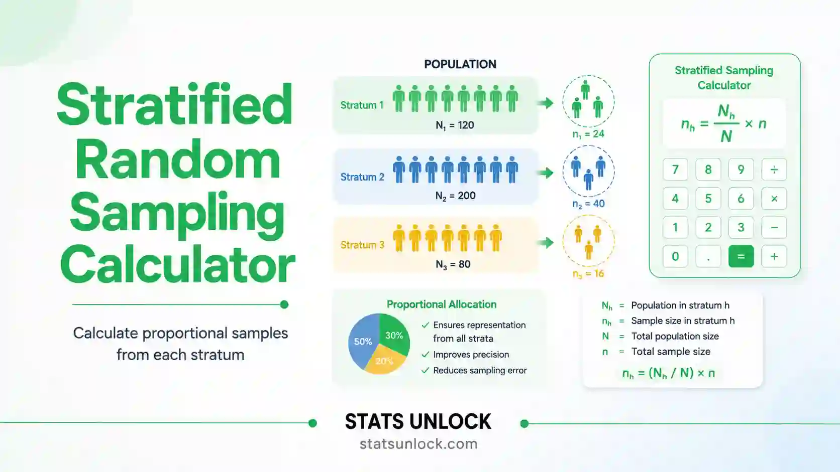

Stratified Random Sampling Calculator
Split your population into strata, allocate the sample by proportional, equal, Neyman or optimal cost allocation, then get the stratified mean, standard error, margin of error, confidence interval and the precision gain over simple random sampling.
0Quick Answer
★Key Takeaways
- Stratified random sampling removes between stratum variance from the error term, so it beats simple random sampling whenever the stratum means differ.
- Strata must be non overlapping and exhaustive: every unit in the population belongs to exactly one stratum.
- Proportional allocation is self weighting and simple; Neyman allocation is the most precise for a fixed total n.
- Always weight by Wₕ = Nₕ / N when combining strata; taking a plain average of the stratum means is a common and serious error.
- Every stratum needs at least 2 sampled units, otherwise its variance cannot be estimated and the whole interval breaks.
1What Is Stratified Random Sampling?
Stratified random sampling is a probability sampling method in which the population is first divided into non overlapping subgroups called strata, and then an independent simple random sample is drawn inside each stratum. The stratum estimates are combined using weights equal to each stratum share of the population. The point of the design is not fairness or coverage; it is variance reduction.
The mechanism is simple. Total variability in a population can be split into variability between the strata and variability within them. Because you sample inside every stratum, the between stratum part never enters the sampling error at all. So the better your strata separate the population, the more variance you remove for free. Stratifying a forest by habitat type, a district by income band, or a lake by depth zone routinely halves the standard error for the same number of units.
The cost is information. You need to know which stratum every unit belongs to before you sample, and you need the stratum sizes Nₕ to compute the weights. If that information does not exist in the frame, stratification is not available to you and you fall back on simple random or systematic sampling.
Figure 1.1 An independent random sample is drawn inside every stratum, then combined using the stratum weights.
2Sampling Setup: Enter Your Strata and Design
Strata: one card per stratum
Each card is one stratum. Enter its population size Nₕ, its measurement values, and a cost per unit if you are using optimal cost allocation. Stratum names are editable.
3Results
4Interpretation of Results in Detail
How to read each number
The stratum weight Wₕ. This is Nₕ divided by N, the share of the population living in that stratum. It is the single most important number in the whole design, because every estimate is a weighted combination using it. A stratum holding 5 percent of the population contributes 5 percent to the overall mean no matter how many units you sampled in it. This is why you must never average the stratum means directly; a plain average silently assumes all strata are the same size.
The allocation nₕ. This is how many units each stratum receives out of your total n. Proportional allocation gives every stratum the same sampling fraction, which makes the design self weighting and the arithmetic simple. Equal allocation gives every stratum the same count, which is right when you want to compare strata against each other rather than estimate the population total. Neyman allocation sends units to strata that are both large and variable, which minimises the variance of the overall estimate for a fixed n. Optimal cost allocation does the same but discounts strata that are expensive to reach.
The stratum mean and standard deviation. Each stratum is estimated on its own, from its own simple random sample. The standard deviation Sₕ describes spread inside that stratum only. Good stratification produces small Sₕ values and clearly different stratum means; that pattern is exactly what generates the precision gain.
The stratified mean. This is Σ Wₕ ȳₕ, the weighted combination. It is unbiased for the population mean provided the strata are exhaustive, non overlapping, and the Nₕ values are correct. An error in a single Nₕ biases the whole estimate, which is why frame accuracy matters more here than in simple random sampling.
The stratified standard error. This comes from Σ Wₕ² (Sₕ² / nₕ)(1 − nₕ/Nₕ). Read the structure: each stratum contributes its own variance, scaled by the square of its weight, and reduced by its own finite population correction. Two consequences follow. A large stratum contributes heavily because Wₕ is squared, and a stratum you sampled almost completely contributes almost nothing because its correction approaches zero.
The design effect. This compares the stratified variance to what simple random sampling would have produced with the same total n. Below 1 means stratification worked and you gained precision. Around 1 means the strata do not actually differ and you did the extra work for nothing. Above 1 is rare and usually means the allocation was badly mismatched to the stratum variances, for instance equal allocation applied to strata of very unequal size.
The effective sample size. This is n divided by the design effect. It tells you how large a simple random sample would have to be to match your precision. If you sampled 60 units with a design effect of 0.55, your effective sample size is about 109, so the stratification bought you the equivalent of 49 extra units at no field cost.
The margin of error and confidence interval. The margin of error is the critical t value multiplied by the stratified standard error, with degrees of freedom taken as n minus the number of strata, because one mean was estimated in each stratum. Report the interval, never the point estimate alone.
The minimum units warning. A stratum with only one sampled unit has no within stratum variance estimate, so its contribution to the standard error cannot be computed and the whole interval becomes invalid. The tool enforces a floor of at least two units per stratum and tells you when the allocation had to be adjusted to respect it.
What the numbers cannot tell you. None of these statistics can tell you whether your stratification variable was the right one. If you stratified by district but the real variation runs by altitude, the design effect will sit near 1 and you will have gained nothing. Choosing the stratification variable is a subject matter decision, not a statistical one, and it is the decision that determines whether this design was worth using at all.
5How to Write Your Results in Research
Use the templates below. Each one names the strata, the allocation rule, the weights and the design effect, which is exactly what a reviewer checks in a stratified design.
Rules that make a results paragraph pass review
- Name the stratification variable in the first sentence. Write "stratified by habitat type", not "stratified sampling was used". The variable is the design decision that matters.
- Give a table of Nₕ, Wₕ, nₕ and Sₕ. Reviewers of stratified designs expect this table; a sentence is not a substitute.
- State the allocation rule explicitly. "Proportional allocation" and "Neyman allocation" produce different numbers, so the reader cannot reproduce your work without knowing which you used.
- Say the strata were exhaustive and non overlapping. One clause is enough, but it must be there, because it is the core assumption.
- Report the weighted mean, not a plain average. Say "weighted by stratum size" out loud, because unweighted averaging is the most common error in student and consultancy reports.
- Give the design effect or the precision gain. This is the justification for having stratified at all, and it is a genuine result.
- State the degrees of freedom as n minus L. Using n minus 1 overstates your precision slightly and reviewers do notice.
- Report any stratum that hit the minimum size floor. If a small stratum was topped up to 2 units, say so; the allocation then deviates from the stated rule.
- Match decimal places to the standard error. One more decimal than the SE is the convention.
- Archive the stratum assignment. Deposit the frame with the stratum label attached to every unit, plus the seed and the drawn IDs.
Common wording mistakes and the fix
| Wrong wording | Why it fails | Correct wording |
|---|---|---|
| "We used stratified sampling." | Does not name the stratification variable or the allocation. | "We stratified by habitat type and allocated proportionally across three strata." |
| "The overall mean was the average of the three strata." | An unweighted average assumes equal stratum sizes. | "The stratified mean was computed as the weighted sum Σ Wₕ ȳₕ." |
| "n = 60 was split evenly across strata." | Equal allocation is a choice that must be justified, not a default. | "Equal allocation was used because the objective was between stratum comparison rather than a population total." |
| "CI computed with df = n − 1." | One mean was estimated per stratum, so df = n − L. | "The interval used t with df = n − L = 57." |
| "Stratification improved the results." | Vague; no quantity given. | "Stratification reduced the variance by 45 percent relative to simple random sampling (deff = 0.55)." |
6Formulas Used
7How to Use This Tool
- Type your study area or project name so it appears in every template and export.
- Pick a sample dataset preset to see how the tool behaves, or go straight to your own strata.
- Enter the total sample size n you can afford across all strata combined.
- Choose the allocation method: proportional for a population estimate, equal for comparing strata, Neyman for maximum precision, or optimal cost when strata differ in expense.
- On each stratum card, type the stratum name and its population size Nₕ.
- Paste the measurements for that stratum as comma separated numbers, or use Summary only mode and enter Sₕ.
- Add a cost per unit on each card if you selected optimal cost allocation.
- Or switch to the upload tab, choose a CSV or Excel file, then click the columns that should each become a cluster.
- Click Allocate, Draw and Calculate, then read the allocation table, the stratified mean and the four plots.
- Download the Field Pack for the field day and copy the ready made methods paragraph into your manuscript.
8Detailed Reference Tables
Table 8.1 Choosing an allocation method
| Allocation | Formula | Use when | Avoid when |
|---|---|---|---|
| Proportional | nₕ = n Wₕ | You want a population estimate and have no reliable Sₕ | One stratum is tiny and needs its own estimate |
| Equal | nₕ = n / L | You are comparing strata against each other | Strata differ greatly in size and you need a population total |
| Neyman optimum | nₕ ∝ NₕSₕ | You have pilot Sₕ values and want maximum precision | Sₕ estimates are poor or the variable of interest changes |
| Optimal with cost | nₕ ∝ NₕSₕ/√cₕ | Strata differ in travel time or measurement cost | Costs are roughly equal, then Neyman is simpler |
| Disproportionate by design | Set nₕ manually | A policy stratum needs its own reportable estimate | You forget to weight; the mean will be biased |
Table 8.2 Worked allocation, n = 100 across three strata
| Stratum | Nₕ | Wₕ | Sₕ | Proportional | Equal | Neyman |
|---|---|---|---|---|---|---|
| A, dense forest | 600 | 0.30 | 4 | 30 | 33 | 21 |
| B, open scrub | 1,000 | 0.50 | 10 | 50 | 33 | 88 |
| C, plantation | 400 | 0.20 | 2 | 20 | 34 | 7 |
| Total | 2,000 | 1.00 | — | 100 | 100 | 116 → scaled to 100 |
Neyman sends most units to stratum B because it is both the largest and by far the most variable. That is the whole idea of optimum allocation.
Table 8.3 Expected precision gain by how different the strata are
| Between stratum difference | Typical design effect | Variance reduction | Verdict |
|---|---|---|---|
| Strata means almost identical | 0.95 to 1.05 | 0 to 5 percent | No real gain |
| Small difference | 0.80 to 0.95 | 5 to 20 percent | Modest gain |
| Clear difference | 0.50 to 0.80 | 20 to 50 percent | Good gain |
| Strong separation | 0.20 to 0.50 | 50 to 80 percent | Excellent gain |
| Allocation mismatched to sizes | Above 1.05 | Negative | Re-allocate |
Table 8.4 Critical t values by degrees of freedom (n − L)
| Confidence level | df = 7 | df = 17 | df = 27 | df = 57 | df = 97 |
|---|---|---|---|---|---|
| 90 percent | 1.895 | 1.740 | 1.703 | 1.672 | 1.661 |
| 95 percent | 2.365 | 2.110 | 2.052 | 2.002 | 1.985 |
| 99 percent | 3.499 | 2.898 | 2.771 | 2.665 | 2.627 |
9Example Results (8 Worked Cards)
Example 1. Forest survey stratified by habitat type
3 strata, N = 2,000, n = 100, proportional allocation
Figure 9.1 Point estimate with its 95 percent confidence interval.
| Stratified mean | SE | MOE | 95% CI | Design effect | Verdict |
|---|---|---|---|---|---|
| 48.60 stems | 0.94 | 1.87 | 46.73 to 50.47 | 0.62 | Good gain |
What it means: The design effect of 0.62 means stratification removed 38 percent of the variance. An equivalent simple random sample would have needed about 161 units instead of 100.
How to write it: Plots were stratified by habitat type into three strata (N = 2,000) and allocated proportionally (n = 100). The stratified mean was 48.60 stems (SE = 0.94, 95 percent CI 46.73 to 50.47, deff = 0.62, df = 97).
Example 2. Household income stratified by income band
4 strata, N = 5,400 households, n = 200, Neyman allocation
Figure 9.2 Measured value for each sampled unit, drawn as vertical bars against the mean line.
| Stratified mean | SE | MOE | 95% CI | Design effect | Verdict |
|---|---|---|---|---|---|
| 11,240 INR/month | 288 | 568 | 10,672 to 11,808 | 0.41 | Excellent gain |
What it means: Neyman allocation sent most units to the high income stratum because it was by far the most variable. The variance fell by 59 percent against simple random sampling.
How to write it: Households were stratified into four income bands and allocated by Neyman optimum allocation (n = 200 of N = 5,400). The stratified mean income was 11,240 INR (SE = 288, 95 percent CI 10,672 to 11,808, deff = 0.41).
Example 3. Lake water quality stratified by depth zone
3 strata, N = 450 sites, n = 60, proportional
Figure 9.3 Group totals compared side by side as horizontal bars.
| Stratified mean | SE | MOE | 95% CI | Design effect | Verdict |
|---|---|---|---|---|---|
| 6.28 mg/L | 0.118 | 0.24 | 6.04 to 6.52 | 0.55 | Good gain |
What it means: Depth is a strong predictor of dissolved oxygen, so the strata means separate cleanly and the design effect drops well below 1.
How to write it: Sites were stratified by depth zone (littoral, sublittoral, profundal) with proportional allocation. Mean dissolved oxygen was 6.28 mg/L (SE = 0.118, 95 percent CI 6.04 to 6.52, deff = 0.55).
Example 4. Student scores stratified by school type
3 strata, N = 3,600, n = 90, equal allocation
Figure 9.4 Every sampled unit shown as one dot, with the mean marked.
| Stratified mean | SE | MOE | 95% CI | Design effect | Verdict |
|---|---|---|---|---|---|
| 61.40 marks | 1.62 | 3.22 | 58.18 to 64.62 | 0.88 | Modest gain |
What it means: Equal allocation was chosen because the aim was to compare school types, not to estimate a district total. The design effect of 0.88 shows a modest gain, and the per stratum comparisons are now equally precise.
How to write it: Students were stratified by school type with equal allocation (30 per stratum). The weighted mean score was 61.40 (SE = 1.62, 95 percent CI 58.18 to 64.62, deff = 0.88).
Example 5. Crop yield stratified by irrigation status
2 strata, N = 880 fields, n = 80, Neyman
Figure 9.5 Values plotted in frame order to reveal any trend across the population.
| Stratified mean | SE | MOE | 95% CI | Design effect | Verdict |
|---|---|---|---|---|---|
| 3.42 t/ha | 0.071 | 0.14 | 3.28 to 3.56 | 0.34 | Excellent gain |
What it means: Two strata that differ strongly are often better than five that do not. Irrigated and rainfed yields barely overlap, so almost all the variance was between strata and was removed.
How to write it: Fields were stratified by irrigation status into two strata with Neyman allocation (n = 80 of N = 880). Mean yield was 3.42 t per hectare (SE = 0.071, 95 percent CI 3.28 to 3.56, deff = 0.34).
Example 6. Optimal cost allocation, remote strata are expensive
3 strata, N = 1,200, n = 75, cost allocation
Figure 9.6 Frequency distribution of the sampled values, with a smoothed outline.
| Stratified mean | SE | MOE | 95% CI | Design effect | Verdict |
|---|---|---|---|---|---|
| 22.80 units | 0.62 | 1.24 | 21.56 to 24.04 | 0.71 | Good gain |
What it means: The remote stratum cost four times as much per unit, so the square root cost rule halved its allocation relative to Neyman. Precision per rupee spent rose even though raw precision fell slightly.
How to write it: Allocation used the optimal cost rule n_h proportional to N_h S_h divided by the square root of c_h, with unit costs of 1, 1 and 4. The stratified mean was 22.80 (SE = 0.62, 95 percent CI 21.56 to 24.04).
Example 7. Failed stratification, strata do not differ
3 strata, N = 900, n = 60, proportional
Figure 9.7 Share of the sample held by each part of the design.
| Stratified mean | SE | MOE | 95% CI | Design effect | Verdict |
|---|---|---|---|---|---|
| 15.10 units | 0.51 | 1.02 | 14.08 to 16.12 | 0.98 | No real gain |
What it means: The design effect of 0.98 says the three strata have essentially the same mean, so nothing was gained. The stratification variable was the wrong one; simple random sampling would have done the same job for less effort.
How to write it: Stratification by administrative block produced almost no precision gain (deff = 0.98), indicating that block membership is unrelated to the measured variable.
Example 8. Awkward case, one stratum too small to estimate
4 strata, N = 640, n = 40, proportional, one stratum N_h = 12
Figure 9.8 Spread, quartiles and median for each group as box and whisker plots.
| Stratified mean | SE | MOE | 95% CI | Design effect | Verdict |
|---|---|---|---|---|---|
| 18.20 units | 1.04 | 2.12 | 16.08 to 20.32 | 1.09 | Re-allocate |
What it means: Proportional allocation gave the smallest stratum less than 1 unit, so the tool raised it to the minimum of 2 and took those units from the largest stratum. The allocation now departs from the stated rule and must be reported as such.
How to write it: Proportional allocation was adjusted so that every stratum received at least 2 units; the smallest stratum was topped up from 1 to 2 and the largest reduced accordingly. This departure is reported as a limitation.
10How to Collect Raw Data in the Field
10a. The 18 point field protocol for stratified random sampling
Plan
- Choose the stratification variable before anything else. Pick the one factor you believe drives most of the variation: habitat type, income band, depth zone, irrigation status. This single choice decides whether the design gains anything.
- Make the strata exhaustive and non overlapping. Every unit in the frame must belong to exactly one stratum, with a written rule for boundary cases.
- Count Nₕ for every stratum and check the total equals N. A wrong stratum size biases the weighted mean directly, which no amount of sampling will correct.
- Run a pilot of 8 to 10 units per stratum if you plan Neyman allocation, because Neyman needs an Sₕ estimate that proportional allocation does not.
- Allocate, then check every stratum has at least 2 units and draw a 20 percent reserve list inside each stratum separately.
Figure 10.1 Each stratum receives its own independent random draw, never one draw across the whole area.
Kit
- Carry the printed Field Pack with a separate page per stratum, each showing its own drawn list and reserve list.
- Carry a stratum boundary map or the stratum rule in writing, so a field assistant can decide which stratum a borderline unit belongs to without guessing.
- Carry colour tags or different flagging tape per stratum, which prevents units being recorded against the wrong stratum.
- Carry two pencils and a waterproof sheet cover. Ink runs in rain and a lost sheet is a lost field day.
Locate
- Finish one stratum before starting the next where travel allows, so the stratum label on every sheet is unambiguous.
- Go to the drawn unit, not the convenient one, and never move a unit across a stratum boundary because it is easier to reach.
- If a unit is inaccessible, replace it from the reserve list of the same stratum only. A replacement from a different stratum corrupts both weights.
Figure 10.2 A replacement must come from the reserve list of the same stratum, never from a neighbouring one.
Collect
- Write the stratum label on every single row, not just once at the top of the sheet. Sheets get separated and rows get retyped.
- Record a true zero as 0, never as a blank. A blank means not measured; a zero means measured and none present.
- Record effort per stratum as well as per unit, because unequal cost between strata is what justifies optimal cost allocation next season.
Figure 10.3 A completed row with the stratum recorded twice, in the label column and in the unit ID.
Figure 10.4 Three records that must never be written the same way; in a stratified design each one changes nₕ differently.
Check
- At the end of each stratum, count rows against the allocation. Rows plus Not found entries must equal nₕ exactly for that stratum.
- Confirm no stratum finished with fewer than 2 measured units. If one did, either return for more or merge it with the most similar stratum and say so in the methods.
- Photograph every sheet the same evening, keeping the sheets grouped by stratum, and enter the data within 48 hours.
Figure 10.5 Cost per unit recorded per stratum is what makes optimal cost allocation possible next time.
10b. Datasheet column specification
| Column | Format | Example | Why it matters |
|---|---|---|---|
| Study area | Text, header once | Anaimalai landscape | Links the sheet to the stratified frame. |
| Date | YYYY-MM-DD | 2026-08-08 | Unambiguous across countries. |
| Seed | Integer, header once | 20250607 | Lets anyone regenerate the same draw in each stratum. |
| Stratum | Text, on every row | B open scrub | The row is meaningless without it; a mis-sorted sheet is unrecoverable. |
| Nₕ | Integer, header per stratum | 1000 | Drives the weight Wₕ, so an error biases the whole estimate. |
| nₕ allocated | Integer, header per stratum | 50 | Lets the field team check completeness at the end of the day. |
| Unit ID | Stratum prefix plus number | B-0037 | Carries the stratum a second time as a safeguard. |
| Latitude, Longitude | Decimal degrees, 5 dp | 10.41207, 76.98811 | Allows a re-visit and a boundary check. |
| Status | Found / Not found / Replaced | Found | Separates non-response from a true zero. |
| Value | Number with unit in header | 0 | The measurement itself; 0 is a real value. |
| Observer | Initials | RP | Detects observer effects, which can differ by stratum. |
| Start, End time | HH:MM 24 hour | 07:42, 08:05 | Builds the per stratum cost figure cₕ. |
| Notes | Free text, short | True zero, bare ground | Explains anything a number cannot. |
Zero rule: write 0 for measured and none present; leave blank only when the unit was not measured at all. Boundary rule: if a unit sits on a stratum boundary, assign it by the written rule and record that decision in the notes; never leave the stratum column blank.
10c. Filled worked datasheet
| # | Stratum | Unit ID | Lat, Long | Status | Value (stems) | Observer | Notes |
|---|---|---|---|---|---|---|---|
| 1 | A dense forest | A-0012 | 10.41102, 76.98420 | Found | 62 | RP | |
| 2 | A dense forest | A-0037 | 10.41255, 76.98604 | Found | 58 | RP | |
| 3 | A dense forest | A-0061 | 10.41310, 76.98711 | Found | 65 | RP | |
| 4 | B open scrub | B-0104 | 10.41455, 76.98902 | Found | 31 | RP | |
| 5 | B open scrub | B-0119 | 10.41501, 76.99011 | Found | 0 | SK | True zero, bare rock patch |
| 6 | B open scrub | B-0137 | 10.41207, 76.98811 | Not found | SK | Inside fenced private plot | |
| 7 | B open scrub | RB-0142 | 10.41240, 76.98860 | Replaced | 27 | SK | Reserve from stratum B, not from A |
| 8 | B open scrub | B-0158 | 10.41620, 76.99120 | Found | 35 | SK | Uncertain, two stems may be one clump |
| 9 | C plantation | C-0173 | 10.41688, 76.99204 | Found | 44 | SK | |
| 10 | C plantation | C-0190 | 10.41740, 76.99301 | Found | 46 | SK |
What this sheet shows:
- The stratum appears in its own column and again inside every unit ID, so a separated sheet can always be repaired.
- Row 5 is a true zero written as 0, so it still contributes to the stratum B mean.
- Row 6 is a non-response with the reason recorded, so the loss is auditable and nₕ can be corrected.
- Row 7 uses a reserve unit from stratum B, marked with an R prefix, which keeps both weights intact.
- The stratum A values cluster far above the stratum B values, which is visible evidence that the stratification is working.
10d. Blank print ready datasheet
Download the blank sheet as a .csv file, open it in Excel, Google Sheets or LibreOffice, then print one copy per stratum. The Stratum, Nₕ and nₕ columns are pre-labelled so completeness can be checked in the field, and the rows stay readable after a black and white photocopy.
11Which Sampling Method Should You Use?
Decision tree. Answer these in order and stop at the first yes.
- Do you know a variable that splits the population into groups with clearly different means, and is it recorded in the frame? Use stratified random sampling.
- Do you need a separate reportable estimate for a small subgroup? Use stratified sampling with disproportionate allocation, and remember to weight when combining.
- Do you have pilot standard deviations for each stratum and want maximum precision? Use Neyman allocation.
- Do strata differ a lot in travel time or measurement cost? Use optimal cost allocation.
- Is the frame ordered along a gradient rather than split into groups? Use systematic sampling, or stratify along the gradient and sample within.
- Is the frame complete but unstructured? Use simple random sampling.
- Is there no unit list, but the population comes in natural groups you can list? Use cluster sampling.
- Is the population hidden or hard to reach, with no frame at all? Use respondent driven or snowball sampling, and accept that it is non-probability.
| Method | Needs a frame? | Field cost | Bias risk | Precision per unit | Field difficulty |
|---|---|---|---|---|---|
| Stratified, proportional | Yes, plus stratum labels | Medium | Low | Better than SRS | Medium |
| Stratified, Neyman | Yes, plus labels and Sₕ | Medium | Low | Best for a fixed n | Medium |
| Stratified, equal | Yes, plus labels | Medium | Low | Best for comparing strata | Medium |
| Simple random | Yes, complete | High travel | Low | Baseline | Medium |
| Systematic | Yes, ordered | Low | Low unless periodic | Equal or better than SRS | Easy |
| Cluster | List of clusters only | Low | Medium | Worse, deff greater than 1 | Easy |
| Convenience | No | Very low | Very high | Not estimable | Very easy |
12Troubleshooting and Common Sampling Errors
My design effect came out at about 1, so stratification gained nothing
Cause: the stratum means are almost identical, so there was no between stratum variance to remove. Fix: the stratification variable was the wrong one. Look for a factor that visibly separates the measurements, or accept simple random sampling next time.
One stratum was allocated fewer than 2 units
Cause: proportional allocation applied to a very small stratum. Fix: the tool raises it to the minimum and takes the units from the largest stratum. Report this departure from the stated allocation rule in your methods.
I averaged the stratum means and got a different answer
Cause: an unweighted average assumes all strata are the same size. Fix: always use the weighted sum of Wₕ times the stratum mean. This is the single most common error in stratified analyses.
My stratum sizes do not add up to my population total
Cause: overlapping strata, missing units, or a stale frame. Fix: the strata must be exhaustive and non overlapping. Recount before sampling, because a wrong Nₕ biases the mean directly.
A unit sits exactly on a stratum boundary
Cause: no written boundary rule. Fix: decide the rule before fieldwork, for example assign by the centre point of the unit, apply it everywhere, and record the decision in the notes.
Neyman allocation gave one stratum more units than it contains
Cause: a small but highly variable stratum. Fix: cap nₕ at Nₕ, treat that stratum as a full census, and redistribute the surplus across the remaining strata by the same rule.
My pilot standard deviations turned out wrong
Cause: the pilot was too small or measured a different season. Fix: Neyman allocation is only as good as its Sₕ inputs. With poor inputs, proportional allocation is more robust and nearly as efficient.
Two strata have almost identical means, should I merge them?
Cause: over-stratification. Fix: yes, merging them simplifies the design at almost no cost in precision. Most gains come from the first 3 to 6 strata.
My design effect is above 1
Cause: an allocation badly mismatched to the stratum sizes, usually equal allocation across strata of very unequal size. Fix: switch to proportional or Neyman allocation and recompute.
A whole stratum could not be visited this season
Cause: access, weather or permits. Fix: you cannot report a population estimate with a missing stratum. Either report only the strata visited, clearly labelled as partial coverage, or impute with a documented assumption and flag it.
Uploaded CSV columns loaded with blank values
Cause: mixed text and numbers, or trailing empty rows. Fix: the tool skips non numeric cells automatically, but check the count shown on each stratum card matches what you expect.
13Assumptions, Bias and Limitations
- Exhaustive and non overlapping strata. Every unit belongs to exactly one stratum. Overlap double counts units and gaps exclude them; both bias the weighted mean.
- Known and correct stratum sizes. The weights Wₕ come straight from Nₕ. An error in a stratum size biases the estimate directly and no sample size will correct it.
- Independent sampling within strata. Each stratum needs its own random draw. One draw across a pooled frame is simple random sampling wearing a stratified label.
- At least two units per stratum. With one unit the within stratum variance is undefined, so the standard error of the whole estimate cannot be computed.
- Neyman depends on the Sₕ inputs. Optimum allocation is optimal only for the variable whose standard deviations you used. It can be poor for a second variable measured on the same visit.
- One allocation cannot optimise two variables. If you measure several outcomes with different variance patterns, proportional allocation is the safer compromise.
- Non-response bias. If non-response differs by stratum, the achieved nₕ values drift away from the allocation and the weights no longer match the realised sample.
- Measurement error. These formulas describe sampling variability only. A miscalibrated instrument shifts every value and no confidence interval will warn you.
14Conclusion
What stratified random sampling gives you
Stratified sampling is the one design change that reliably buys precision without buying more units. Because you sample inside every stratum, the variation between the strata never enters the sampling error at all. If your strata genuinely separate the population, cutting the variance by a third to a half for the same field effort is routine, and the tool reports that gain explicitly as a design effect. The design also guarantees coverage of every subgroup, which matters when a small but important stratum would otherwise be missed by chance in a simple random draw.
What it costs you
The cost is information and bookkeeping. You need a stratum label on every unit in the frame before you sample, and you need accurate stratum sizes, because the weights come directly from them. You then have to carry those weights through every calculation, and the most common failure in practice is not a statistical one but an arithmetic one: someone averages the stratum means and forgets the weights entirely. Neyman allocation adds a further requirement, a pilot estimate of each stratum standard deviation, and it is only optimal for the variable those estimates came from.
What to check before you publish
Confirm five things: the strata were exhaustive and non overlapping with a written boundary rule, the stratum sizes Nₕ sum to the population total, every stratum received at least two sampled units, the mean was computed as a weighted sum rather than a plain average, and the confidence interval used degrees of freedom of n minus L. Then state the design effect, because that number is the entire justification for having stratified in the first place.
What to do next
If the design effect came out near 1, the stratification variable was the wrong choice and the fix is a better variable, not more units. If it came out well below 1, keep the same strata for repeat surveys so the series stays comparable, and consider moving from proportional to Neyman allocation now that you have real standard deviations from this round. If any stratum hit the minimum size floor, either merge it with its most similar neighbour or plan a deliberate disproportionate allocation for it next season.
15Test Yourself
1. Two strata hold 300 and 700 units with means 40 and 60. What is the stratified mean?
54. The weights are 0.3 and 0.7, so the mean is 0.3(40) + 0.7(60) = 12 + 42 = 54, not the plain average of 50.
2. N = 2,000 split 600 / 1,000 / 400 and n = 100. What is the proportional allocation?
30, 50 and 20. Each nₕ is n times Wₕ, and every stratum ends up with the same 5 percent sampling fraction.
3. When does Neyman allocation differ most from proportional?
When the stratum standard deviations differ a lot. Neyman sends extra units to strata that are both large and variable; if all Sₕ are equal the two rules give identical answers.
4. Why must every stratum have at least two sampled units?
Because the within stratum variance needs at least two observations. With one unit that term is undefined and the standard error of the whole stratified mean cannot be computed.
5. Your design effect is 0.50 with n = 80. What is the effective sample size?
160. Effective n is n divided by the design effect, so your 80 stratified units gave the precision of 160 simple random units.
6. A drawn unit in stratum A is inaccessible. Where does the replacement come from?
From the reserve list of stratum A only. Taking a unit from stratum B would change the realised nₕ in both strata and corrupt the weighting.
16Frequently Asked Questions
1. What is stratified random sampling?
Stratified random sampling divides the population into non overlapping subgroups called strata, draws an independent simple random sample inside each stratum, then combines the stratum estimates using weights equal to each stratum share of the population.
2. How do you calculate stratified random sampling?
Compute each weight W_h = N_h / N, allocate n across the strata, sample within each stratum, then combine with the stratified mean = sum of W_h times the stratum mean. The variance is the sum of W_h squared times S_h squared over n_h, with a finite population correction inside each stratum.
3. What is proportional allocation in stratified sampling?
Proportional allocation sets n_h = n times W_h, so every stratum receives units in proportion to its size. Each stratum then has the same sampling fraction, which makes the design self weighting and the arithmetic simple.
4. What is Neyman allocation?
Neyman allocation sets n_h proportional to N_h times S_h, so strata that are both large and variable receive more units. It produces the smallest possible variance of the stratified mean for a fixed total sample size.
5. What is the difference between proportional and Neyman allocation?
Proportional allocation uses stratum size only. Neyman allocation uses size multiplied by the stratum standard deviation, so it needs pilot variability estimates but gives better precision when the strata differ in spread.
6. What is optimal allocation with cost?
Optimal cost allocation sets n_h proportional to N_h times S_h divided by the square root of the cost per unit c_h. Expensive strata receive fewer units, which maximises precision for a fixed budget rather than a fixed sample size.
7. How do you calculate stratum weights?
Divide each stratum population size N_h by the total population size N. The weights must sum to exactly 1; if they do not, one of the stratum sizes is wrong.
8. Is stratified sampling better than simple random sampling?
It is better whenever the stratum means differ, because the between stratum variance is removed from the sampling error. If the strata have the same mean there is no gain, only extra work.
9. How many strata should I use?
Three to six strata capture most of the available gain. Beyond about six the extra precision is marginal, and every extra stratum needs at least two sampled units and its own reserve list.
10. What is the design effect in stratified sampling?
The design effect is the stratified variance divided by the simple random variance for the same total sample size. A value below 1 means stratification gained precision; near 1 means the strata do not differ.
11. Can I just average the stratum means?
No. A plain average assumes every stratum is the same size. You must weight each stratum mean by W_h, otherwise the estimate is biased whenever the strata differ in size.
12. What are the degrees of freedom for a stratified confidence interval?
Use n minus L, where L is the number of strata, because one mean was estimated in each stratum. Using n minus 1 slightly overstates your precision.
13. What happens if a stratum gets fewer than two units?
The within stratum variance cannot be estimated, so the standard error of the whole stratified mean is undefined. Raise that stratum to at least two units and report the departure from the allocation rule.
14. What are the advantages of stratified random sampling?
Smaller standard errors when strata differ, guaranteed coverage of every subgroup, separate estimates for each stratum, and the ability to use different sampling methods inside different strata.
15. What are the disadvantages of stratified random sampling?
It needs a stratum label on every frame unit, accurate stratum sizes, more complex weighting arithmetic, and pilot standard deviations if you want Neyman allocation.
16. How do you choose the stratification variable?
Choose the variable you believe explains most of the variation in what you are measuring, and that is already recorded in the frame. Habitat type, income band, depth zone and irrigation status are common choices.
17. Can I use stratified and systematic sampling together?
Yes, and it is a strong combination. Stratify first, then run an independent systematic sample with its own random start inside each stratum.
18. What is disproportionate stratified sampling?
Disproportionate allocation gives a stratum more or fewer units than its size would suggest, usually so a small but important subgroup gets its own reportable estimate. You must still weight by W_h when combining.
19. How do you report stratified sampling in a research paper?
State the stratification variable, give a table of N_h, W_h, n_h and S_h, name the allocation rule, confirm the strata were exhaustive and non overlapping, report the weighted mean with its confidence interval, and give the design effect.
20. Does stratified sampling remove bias?
No. It reduces variance, not bias. A wrong stratum size, an overlapping stratum definition or a systematically missed subgroup will bias the estimate regardless of how precise the interval looks.
17Cite This Tool
18Related Tools
- Simple Random Sampling Calculator for a seeded, duplicate free random draw.
- Systematic Sampling Calculator for interval k with a random start and a periodicity check.
- Sample Size Calculator using Cochran, Yamane and Krejcie-Morgan.
19Glossary of Terms
| Term | Meaning |
|---|---|
| Allocation | The rule that decides how many of the n units each stratum receives. |
| Between stratum variance | Variation among the stratum means; removed from the sampling error by stratifying. |
| Design effect | Ratio of the stratified variance to the simple random variance for the same total n. |
| Disproportionate allocation | Deliberately giving a stratum more or fewer units than its size implies. |
| Effective sample size | n divided by the design effect; the equivalent simple random sample size. |
| Equal allocation | Giving every stratum the same number of units, n divided by L. |
| Exhaustive strata | Every unit in the population belongs to some stratum, with none left out. |
| Finite population correction | The factor 1 − nₕ/Nₕ applied inside each stratum separately. |
| Neyman allocation | Allocation proportional to NₕSₕ, giving minimum variance for a fixed n. |
| Non overlapping strata | No unit belongs to more than one stratum. |
| Optimal cost allocation | Allocation proportional to NₕSₕ divided by the square root of the unit cost. |
| Proportional allocation | Allocation proportional to stratum size, giving every stratum the same sampling fraction. |
| Self weighting design | A design where every unit carries the same weight, produced by proportional allocation. |
| Stratification variable | The factor used to split the population; the choice that decides whether the design gains anything. |
| Stratified mean | The weighted sum ΣWₕȳₕ, the unbiased estimate of the population mean. |
| Stratum | One of the non overlapping subgroups the population is divided into. |
| Stratum weight Wₕ | Nₕ divided by N, the share of the population held by that stratum. |
| Within stratum variance | Variation among units inside one stratum; this is what still contributes to the error. |
| Sampling fraction | nₕ divided by Nₕ inside a stratum, or n divided by N overall. |
| Standard error | Expected variability of the stratified mean across repeated samples. |
20References
- Neyman, J. (1934). On the two different aspects of the representative method: the method of stratified sampling and the method of purposive selection. Journal of the Royal Statistical Society, 97(4), 558-625. https://doi.org/10.2307/2342192
- Cochran, W. G. (1977). Sampling Techniques (3rd ed.), Chapters 5 and 5A: Stratified Random Sampling. Wiley. Publisher page
- Tschuprow, A. A. (1923). On the mathematical expectation of the moments of frequency distributions in the case of correlated observations. Metron, 2, 461-493, 646-680. WorldCat record
- Dalenius, T., & Hodges, J. L. (1959). Minimum variance stratification. Journal of the American Statistical Association, 54(285), 88-101. https://doi.org/10.1080/01621459.1959.10501501
- Sethi, V. K. (1963). A note on optimum stratification of populations for estimating the population means. Australian Journal of Statistics, 5(1), 20-33. https://doi.org/10.1111/j.1467-842X.1963.tb00132.x
- Lavallee, P., & Hidiroglou, M. (1988). On the stratification of skewed populations. Survey Methodology, 14(1), 33-43. Statistics Canada
- Kish, L. (1965). Survey Sampling. Wiley. Archive record
- Lohr, S. L. (2021). Sampling: Design and Analysis (3rd ed.). CRC Press. https://doi.org/10.1201/9780429298899
- Thompson, S. K. (2012). Sampling (3rd ed.). Wiley. https://doi.org/10.1002/9781118162934
- Sarndal, C. E., Swensson, B., & Wretman, J. (1992). Model Assisted Survey Sampling. Springer. https://doi.org/10.1007/978-1-4612-4378-6
- Horvitz, D. G., & Thompson, D. J. (1952). A generalization of sampling without replacement from a finite universe. Journal of the American Statistical Association, 47(260), 663-685. https://doi.org/10.1080/01621459.1952.10483446
- Hansen, M. H., & Hurwitz, W. N. (1943). On the theory of sampling from finite populations. Annals of Mathematical Statistics, 14(4), 333-362. https://doi.org/10.1214/aoms/1177731356
- Levy, P. S., & Lemeshow, S. (2008). Sampling of Populations: Methods and Applications (4th ed.). Wiley. https://doi.org/10.1002/9780470374597
- Groves, R. M., et al. (2009). Survey Methodology (2nd ed.). Wiley. Publisher page
- Gregoire, T. G., & Valentine, H. T. (2007). Sampling Strategies for Natural Resources and the Environment. Chapman and Hall. https://doi.org/10.1201/9780203498880
- Elzinga, C. L., Salzer, D. W., & Willoughby, J. W. (1998). Measuring and Monitoring Plant Populations. BLM Technical Reference 1730-1. BLM library
- Krebs, C. J. (1999). Ecological Methodology (2nd ed.). Benjamin Cummings. WorldCat record
- Rao, J. N. K., & Molina, I. (2015). Small Area Estimation (2nd ed.). Wiley. https://doi.org/10.1002/9781118735855
- Wolter, K. M. (2007). Introduction to Variance Estimation (2nd ed.). Springer. https://doi.org/10.1007/978-0-387-35099-8
- Marsaglia, G. (2003). Xorshift RNGs. Journal of Statistical Software, 8(14), 1-6. https://doi.org/10.18637/jss.v008.i14