In a right skewed distribution is the mean greater than the median?

Yes. In a right skewed distribution the mean is usually greater than the median because extreme high values in the right tail pull the mean upward while the median stays near the bulk of the data.

What skewness value is acceptable for normality?

A common rule is that skewness between -0.5 and +0.5 is approximately symmetric, between 0.5 and 1 (or -1 and -0.5) is moderately skewed, and beyond plus or minus 1 is highly skewed. Values within about plus or minus 2 are often treated as acceptable for many parametric analyses.

Right Skewed vs Left Skewed: Difference, Examples & Calculator

Right Skewed vs Left Skewed: Free Skewness Calculator & Guide

Right Skewed vs Left Skewed: Skewness Calculator with Plots & Interpretation

Paste your data or upload a CSV file and instantly find out whether your distribution is right skewed (positive skew) or left skewed (negative skew). Get the skewness value, standard error, four colorful plots, and ready-to-copy sentences for your research paper.

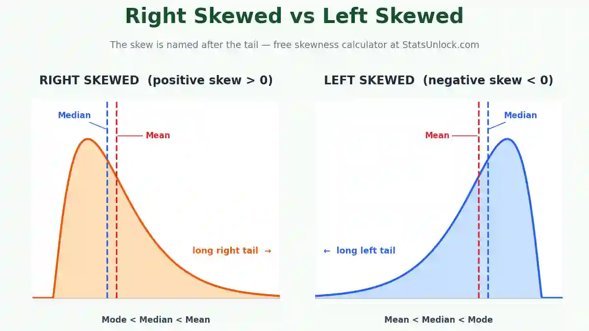
Descriptive StatisticsSkewnessDistribution ShapeFree Online Tool

Quick answer: A right skewed (positively skewed) distribution has a long tail on the right side — most values are low, the mean is greater than the median, and skewness is above 0. A left skewed (negatively skewed) distribution has a long tail on the left side — most values are high, the mean is less than the median, and skewness is below 0. The skew is always named after the direction of the tail.

🔑 Key Takeaways

1The skew is named after the tail, not the peak. A right skewed distribution has its long tail pointing right (toward large values); a left skewed distribution has its long tail pointing left.
2Right skewed = positive skew (> 0); left skewed = negative skew (< 0). "Positively skewed" and "right skewed" are the same thing — just two names for one shape.
3The mean chases the tail. In right skewed data: mode < median < mean. In left skewed data the order reverses. Comparing mean and median is the fastest skew check without any formula.
4Use the benchmark ranges to judge severity. Skewness within ±0.5 is approximately symmetric, ±0.5 to ±1 is moderate, and beyond ±1 is highly skewed.
5Test significance with z = skewness ÷ SES. If |z| > 1.96 the skew is significant at α = 0.05 — but at large n (> 300), judge by the value and the plots instead, because tiny skews turn "significant."
6Skewed data change what you should report and run. For clearly skewed variables, report the median and IQR instead of mean and SD, and prefer transformations, non-parametric tests, or GLMs over plain t-tests in small samples.
7Zero skewness does not prove normality. Symmetric bimodal or heavy-tailed data also score near zero — always pair the skewness number with a histogram, Q-Q plot, kurtosis, and a normality test.

📥 Enter Your Data

Comma-separated input is the default. You can also separate values with spaces, semicolons, or new lines. The group name is editable — click it and type your own label.

Upload CSV file (.csv, .txt)

Headers are detected automatically. Click the columns that should each become a cluster — every selected column is loaded as its own separate group.

🛠 How to Use This Skewness Calculator

Enter your data. Paste comma-separated values (e.g., 52, 48, 55, 61, 47), load one of the five sample datasets, or upload a CSV file and click the columns you want loaded as separate clusters.
Name your groups. Click any group name to edit it, and use + Add Group to compare several variables side by side.
Click "Calculate Skewness." The tool computes the Fisher-Pearson g₁, the adjusted G₁ (matches SPSS, Excel, and R), Pearson's second coefficient, the standard error, and the z-test.
Read the direction. Skewness > 0 means right skewed (positive skew); < 0 means left skewed (negative skew); within ±0.5 is approximately symmetric.
Verify with the plots and report. Check the histogram, box plot, mean-vs-median plot, and Q-Q plot, then copy an APA-style template from the reporting section into your paper.

↔ Right Skewed vs Left Skewed: The Core Difference

The fastest way to remember right skewed vs left skewed is this: the skew is named after the tail, not the peak. A right skewed distribution has its long, thin tail stretching to the right (toward large values). A left skewed distribution has its long tail stretching to the left (toward small values). People search this both ways — left skewed vs right skewed, left skew vs right skew, left vs right skewed — and the answer is always the same: look at the tail.

Feature	Right Skewed (Positive Skew)	Left Skewed (Negative Skew)
Tail direction	Long tail to the right	Long tail to the left
Skewness value	Greater than 0	Less than 0
Typical order	Mode < Median < Mean	Mean < Median < Mode
Mean vs median	Mean pulled above the median	Mean pulled below the median
Real examples	Income, house prices, reaction times, hospital stays	Age at death, easy exam scores, retirement age
Common fix	Log, square-root, or reciprocal transformation	Reflect then transform, or square / cube values

Note that a "skewer" is a kitchen tool, not a statistic — but if your data looks like it was stabbed by one, with a sharp peak and a long tail, it is probably skewed. The word "skewed" simply means the distribution is not symmetric.

ƒ Formulas Used

①

Sample Mean

x̄ = Σxᵢ ÷ n

xᵢEach individual value in your dataset

nNumber of observations in the group

②

Sample Standard Deviation

s = √[ Σ(xᵢ − x̄)² ÷ (n − 1) ]

x̄Sample mean from formula 1

n−1Bessel's correction for an unbiased variance estimate

③

Fisher-Pearson Skewness (g₁)

g₁ = [ Σ(xᵢ − x̄)³ / n ] ÷ [ Σ(xᵢ − x̄)² / n ]^3/2

g₁Moment-based skewness — positive means right skewed, negative means left skewed

m₃Third central moment (numerator) — captures asymmetry direction

m₂Second central moment — standardizes so the result is unitless

④

Adjusted Skewness (G₁) — SPSS / Excel / R default

G₁ = g₁ × √[ n(n − 1) ] ÷ (n − 2)

G₁Small-sample bias-corrected skewness reported by SPSS, Excel, and R (type 2)

Rule|G₁| < 0.5 approx. symmetric · 0.5–1 moderate · > 1 highly skewed

⑤

Pearson's Second Coefficient of Skewness

Sk₂ = 3 × (x̄ − median) ÷ s

Sk₂Quick mean-median comparison — positive when the mean sits above the median (right skew)

sSample standard deviation from formula 2

⑥

Standard Error of Skewness

SES = √[ 6n(n − 1) ÷ ( (n − 2)(n + 1)(n + 3) ) ]

SESUncertainty of the skewness estimate — shrinks as n grows

NoteA rough shortcut is √(6/n) for large samples

⑦

Skewness z-Score (Significance Test)

z = G₁ ÷ SES

zHow many standard errors the skewness lies from zero

Rule|z| > 1.96 → skewness significantly different from 0 at α = 0.05

🔍 Detailed Interpretation of Results

Interpreting skewness is a three-step process: read the sign, read the magnitude, then read the significance. The sign tells you the direction of asymmetry. A positive value means your data are right skewed — most observations sit at the low end and a minority of large values stretch the right tail. A negative value means your data are left skewed — most observations sit at the high end and a minority of small values stretch the left tail. A value close to zero suggests the distribution is roughly symmetric, though symmetry alone does not guarantee normality (a symmetric bimodal distribution also has skewness near zero).

Step 1 — Magnitude benchmarks (Bulmer, 1979 convention)

Skewness (G₁)	Interpretation	Practical meaning
−0.5 to +0.5	Approximately symmetric	Mean and median nearly agree; parametric tests are usually safe on this criterion
+0.5 to +1.0	Moderately right skewed	Mean noticeably above median; check outliers, consider reporting the median
−1.0 to −0.5	Moderately left skewed	Mean noticeably below median; a ceiling effect is a common cause
> +1.0	Highly right skewed	Strong right tail; consider log or square-root transformation, or non-parametric methods
< −1.0	Highly left skewed	Strong left tail; consider reflecting the variable then transforming

Step 2 — Statistical significance

Divide the skewness by its standard error to get the z-score. If |z| exceeds 1.96 the skewness is significantly different from zero at the 5% level; if it exceeds 2.58 it is significant at the 1% level. Be careful with this rule at large sample sizes: with n above roughly 300, even a trivially small skewness becomes "significant," so at large n you should judge by the absolute skewness value and by visual inspection of the histogram and Q-Q plot rather than the z-test (Kim, 2013).

Step 3 — Consequences for your analysis

Skewness matters because many statistical procedures — t-tests, ANOVA, OLS regression, Pearson correlation — assume approximately normal (and therefore symmetric) residuals or sampling distributions. Mild skewness rarely causes problems when samples are moderate to large, thanks to the Central Limit Theorem. Strong skewness, however, distorts the mean, inflates or deflates Type I error rates in small samples, and makes standard deviations misleading. For right skewed data, report the median and interquartile range instead of the mean and SD, or transform the data (log for multiplicative processes such as income or reaction time; square root for counts). For left skewed data, reflect the variable (subtract each value from max + 1) and then apply the same transformations, or use rank-based methods such as the Mann-Whitney or Kruskal-Wallis tests. If interpretation on the original scale matters, generalized linear models (Gamma for right skewed positive data) are often preferable to transformation.

Reading the four plots

The histogram with density curve shows where the tail points: tail right means right skewed, tail left means left skewed. The box plot shows skew through asymmetric whiskers and the median line sitting off-center inside the box — median near the bottom of the box with a long upper whisker signals right skew. The mean vs median plot makes the classic ordering visible: the mean marker to the right of the median marker means right skew; to the left means left skew. The normal Q-Q plot bends above the reference line at the upper end for right skewed data and sags below the line at the lower end for left skewed data; points hugging the line indicate near-symmetry.

✍ How to Write Your Results in Research

Skewness is normally reported inside the descriptive statistics or assumption-checking paragraph of the Results section, alongside kurtosis and a normality test. Always report the statistic, its standard error, and how you judged it. Below are copy-ready templates in APA style — replace the bracketed values with the numbers from the results table above.

Template 1 — Approximately symmetric data

"The distribution of [variable] was approximately symmetric, with skewness of [0.21] (SE = [0.34]). The skewness z-score ([0.62]) did not exceed ±1.96, indicating no significant departure from symmetry; therefore, parametric analyses were considered appropriate."

Template 2 — Right skewed data

"[Variable] was positively (right) skewed, skewness = [1.42] (SE = [0.30]), z = [4.73], p < .05, with the mean ([M] = [312.4]) exceeding the median ([Mdn] = [268.0]). A log₁₀ transformation reduced skewness to [0.18]; transformed values were used in all subsequent parametric analyses."

Template 3 — Left skewed data

"Scores on [variable] showed a negative (left) skew, skewness = [−1.08] (SE = [0.28]), z = [−3.86], reflecting a ceiling effect. Given the departure from symmetry, medians are reported and group comparisons were conducted with the Mann-Whitney U test."

Template 4 — Comparing two groups or clusters

"Skewness differed in direction between groups: [Group A] was right skewed ([0.94], SE = [0.31]) whereas [Group B] was approximately symmetric ([−0.12], SE = [0.29]). Distributional differences were therefore examined with rank-based methods."

Reporting checklist

Report the skewness value to two decimals; include the standard error in parentheses; state the decision rule you used (benchmark ranges or the z-test); mention the sample size, since the reliability of skewness depends heavily on n; and pair the number with a plot (histogram or Q-Q) in the manuscript or supplement, because reviewers trust pictures as much as statistics. If you transformed the data, report skewness before and after transformation.

🔬 Example Results

Below are five worked examples using the built-in sample datasets (each n = 25). Every example shows the distribution shape, the skewness statistics you would get from this calculator, and a ready-made interpretation. Load any of these from the sample dropdown above to reproduce the numbers exactly.

Example 1 — Reaction Times: Right Skewed (Positive Skew)

n = 25 · Mean = 257.16 · Median = 218 · SD = 91.41
Skewness G₁ = 1.78 · SES = 0.46 · z = 3.83

The skewness of 1.78 is well above the +1 benchmark and the z-score (3.83) exceeds 1.96, so the right skew is both strong and statistically significant. The mean (257 ms) sits far above the median (218 ms) because a few very slow responses stretch the right tail — the classic reaction-time pattern. Report the median, or log-transform before running t-tests.

Example 2 — Exam Scores: Left Skewed (Negative Skew)

n = 25 · Mean = 84.52 · Median = 89 · SD = 12.70
Skewness G₁ = −2.08 · SES = 0.46 · z = −4.49

A skewness of −2.08 signals strong left skew — a ceiling effect. Most students scored near the top (median 89) while a few low scores (45, 55, 61) drag the mean down to 84.5 and stretch the left tail. Rank-based tests or a reflect-and-log transformation are appropriate here.

Example 3 — Adult Heights: Approximately Symmetric

n = 25 · Mean = 170.08 · Median = 170 · SD = 3.00
Skewness G₁ = −0.07 · SES = 0.46 · z = −0.16

Skewness of −0.07 sits comfortably inside the ±0.5 symmetric range and the z-score is nowhere near ±1.96. Mean and median agree to within 0.1 cm. This bell-shaped pattern is typical of biological measurements — parametric tests are fully appropriate on the skewness criterion.

Example 4 — Household Income: Strong Right Skew with Outliers

n = 25 · Mean = 60.80 · Median = 43 · SD = 51.51
Skewness G₁ = 2.82 · SES = 0.46 · z = 6.07

With skewness of 2.82, this is extreme right skew driven by three high earners (120k, 180k, 250k). The mean (60.8k) is over 40% higher than the median (43k) — reporting the mean alone would badly misrepresent the typical household. Use the median and IQR, or a log transformation; this is exactly why economists report median income.

Example 5 — Battery Lifespans: Moderate-to-Strong Left Skew

n = 25 · Mean = 96.00 · Median = 98 · SD = 8.01
Skewness G₁ = −1.53 · SES = 0.46 · z = −3.31

Skewness of −1.53 shows meaningful left skew: most batteries last close to their design limit (median 98 hrs) while a few early failures (72, 79, 85 hrs) form the left tail. In reliability work this pattern often calls for a Weibull model rather than a normal one; for simple comparisons, use rank-based tests.

🧭 When to Use This Tool

Use this skewness calculator whenever you need to check distribution shape before choosing a statistical test, describe your data in a thesis or paper, decide whether the mean or the median is the honest summary of your data, screen variables before regression or ANOVA, or teach the difference between right skewed and left skewed distributions. It is designed for researchers, students, data analysts, and instructors, and works with any continuous or discrete numeric variable — reaction times, incomes, test scores, species counts, body measurements, waiting times, and more.

⚠ Assumptions & Limitations

Skewness assumes your data are measured on at least an interval scale and come from a single meaningful group — mixing two populations can fake symmetry or fake skewness. The statistic is highly sensitive to outliers: one extreme value can dominate the third moment, so always inspect the plots. Skewness estimates from small samples (n < 30) are unstable, with wide standard errors; treat them as descriptive only. Zero skewness does not prove normality — check kurtosis and run a Shapiro-Wilk test as well. Finally, different software uses different formulas (g₁ vs G₁ vs b₁); this tool reports both the moment coefficient g₁ and the adjusted G₁ used by SPSS, Excel, and R so your numbers match your software.

🏁 Conclusion

The right skewed vs left skewed distinction comes down to one visual cue and one number. Visually, the skew is named for the tail: a long right tail means right skewed (positive skew), a long left tail means left skewed (negative skew). Numerically, a skewness statistic above zero means right skew, below zero means left skew, and the size of the value tells you how serious the asymmetry is — within ±0.5 is effectively symmetric, beyond ±1 is strongly skewed.

Why does this matter in practice? Because skewness decides which summary statistics and which tests you can trust. In a right skewed distribution the mean is dragged above the median by a few large values, so reporting the mean alone exaggerates the typical case — this is why median income, not mean income, is the standard economic headline. In a left skewed distribution the opposite occurs, often through ceiling effects such as easy exams where most students score near the maximum. Strongly skewed data violate the symmetry expectations behind t-tests, ANOVA, and OLS regression in small samples, and the remedies are well established: transform the data (log or square root for right skew, reflect-then-transform for left skew), switch to rank-based non-parametric tests, or model the skew directly with a generalized linear model.

This calculator gives you everything needed to make and defend that decision: the Fisher-Pearson and adjusted skewness coefficients, Pearson's mean-median coefficient, the standard error and z-test, four diagnostic plots, and APA-style sentences ready to paste into your Results section. Run your data, look at the tail, and let the number confirm what the picture shows — that is all "right skewed vs left skewed" ever asks of you.

❓ Frequently Asked Questions

What is the difference between right skewed and left skewed?

A right skewed distribution has a long tail on the right, with most values at the low end and mean > median. A left skewed distribution has a long tail on the left, with most values at the high end and mean < median. The skew is always named after the direction of the tail.

Is right skewed positive or negative skew?

Right skewed is positive skew (skewness > 0). Left skewed is negative skew (skewness < 0). "Positively skewed" and "right skewed" mean exactly the same thing.

How do I tell if data is skewed left or right from a histogram?

Look for the longer, thinner tail. If it stretches toward larger values on the right, the data are right skewed. If it stretches toward smaller values on the left, the data are left skewed.

In a right skewed distribution, where are the mean, median, and mode?

Typically mode < median < mean. The mode sits at the peak, and the mean is pulled furthest into the right tail by the large values. In left skewed data the order reverses: mean < median < mode.

What skewness value is acceptable for a normal distribution?

Values between −0.5 and +0.5 are treated as approximately symmetric. Many applied researchers accept anything within ±1, and some fields tolerate up to ±2 for large samples. Beyond ±2, transformation or non-parametric methods are strongly recommended.

What are real-life examples of right skewed data?

Household income, house prices, reaction times, hospital length of stay, insurance claims, city population sizes, and social media follower counts are all classically right skewed — most cases are small, a few are extremely large.

What are real-life examples of left skewed data?

Age at death in developed countries, scores on an easy exam, retirement age, and time-to-failure of highly reliable products are typically left skewed — most cases cluster near a high maximum with a minority trailing off to the left.

How do I fix right skewed data?

The most common remedies are the log transformation (best for multiplicative data such as income), the square-root transformation (good for counts), the reciprocal transformation for extreme skew, or switching to non-parametric tests or a Gamma GLM that models the skew directly.

How do I fix left skewed data?

Reflect the variable first — subtract every value from (maximum + 1) so the skew becomes right-sided — then apply a log or square-root transformation. Remember to reverse the interpretation of the transformed scale.

Does skewness of zero mean my data are normal?

No. Zero skewness only means the distribution is symmetric. A bimodal or heavy-tailed symmetric distribution also has skewness near zero. Check kurtosis, a histogram, a Q-Q plot, and a Shapiro-Wilk test before concluding normality.

Can I use a t-test on skewed data?

For mild skew and moderate-to-large samples (n ≥ 30 per group), yes — the Central Limit Theorem protects the t-test. For strong skew with small samples, use the Mann-Whitney U or Wilcoxon test, or transform the data first.

What does a right skewed box plot look like?

The median line sits closer to the bottom of the box, the upper whisker is longer than the lower whisker, and high-end outlier points often appear above the upper whisker.

How large should my sample be for a reliable skewness estimate?

Skewness stabilizes with sample size. Below n = 30 the estimate is very noisy; n ≥ 50 gives a usable estimate; n ≥ 100 or more is ideal if you plan to test the skewness statistically.

Is "skewer" related to skewness?

No — a skewer is a cooking implement. In statistics the correct terms are "skewed," "skewness," "right skewed / positively skewed," and "left skewed / negatively skewed." The shared root simply means "slanted or off-line."

What is the difference between skewness and kurtosis?

Skewness measures asymmetry — whether the tail points left or right. Kurtosis measures tail heaviness — how extreme the outliers are compared with a normal distribution. A distribution can be symmetric (zero skew) yet still have very heavy tails (high kurtosis), so always check both.

Is left skewed the same as left tailed?

Essentially yes in everyday usage: a left skewed distribution has its long tail on the left, so it is sometimes called left tailed. Be careful in hypothesis testing, though — "left-tailed test" refers to the rejection region of a test, not the shape of the data.

What causes right skewed data?

Right skew usually appears when values have a natural floor (often zero) but no ceiling — incomes, waiting times, reaction times, and counts cannot go below zero but a few cases can be enormous. Multiplicative growth processes also produce right skew, which is why the log transformation works so well.

What causes left skewed data?

Left skew usually comes from a ceiling effect — a natural upper limit that most cases approach. Easy exams (many scores near 100%), age at death in wealthy countries, and time-to-failure of highly reliable products all pile up near the maximum with a minority trailing left.

Is a right skewed distribution the same as a positively skewed distribution?

Yes — "right skewed" and "positively skewed" are two names for exactly the same shape: a long tail toward larger values and skewness greater than zero. Likewise "left skewed" equals "negatively skewed." Different textbooks simply prefer different terms.

Can skewness be calculated in Excel, SPSS, or R, and will it match this tool?

Yes. Excel's SKEW(), SPSS's Descriptives, and R's e1071::skewness(type = 2) all report the adjusted Fisher-Pearson coefficient G₁, which is exactly what this calculator reports, so the numbers will match. R's default type 3 and Python's scipy.stats.skew (bias = True) report the moment coefficient g₁, which this tool also displays.

📚 References

Joanes, D. N., & Gill, C. A. (1998). Comparing measures of sample skewness and kurtosis. Journal of the Royal Statistical Society: Series D (The Statistician), 47(1), 183–189. https://doi.org/10.1111/1467-9884.00122
Kim, H.-Y. (2013). Statistical notes for clinical researchers: Assessing normal distribution using skewness and kurtosis. Restorative Dentistry & Endodontics, 38(1), 52–54. https://doi.org/10.5395/rde.2013.38.1.52
Doane, D. P., & Seward, L. E. (2011). Measuring skewness: A forgotten statistic? Journal of Statistics Education, 19(2). https://doi.org/10.1080/10691898.2011.11889611
Bulmer, M. G. (1979). Principles of Statistics. Dover Publications. Publisher page
Blanca, M. J., Arnau, J., López-Montiel, D., Bono, R., & Bendayan, R. (2013). Skewness and kurtosis in real data samples. Methodology, 9(2), 78–84. https://doi.org/10.1027/1614-2241/a000057
Curran, P. J., West, S. G., & Finch, J. F. (1996). The robustness of test statistics to nonnormality and specification error in confirmatory factor analysis. Psychological Methods, 1(1), 16–29. https://doi.org/10.1037/1082-989X.1.1.16
West, S. G., Finch, J. F., & Curran, P. J. (1995). Structural equation models with nonnormal variables: Problems and remedies. In R. H. Hoyle (Ed.), Structural Equation Modeling: Concepts, Issues, and Applications (pp. 56–75). Sage. APA PsycNet record
Tabachnick, B. G., & Fidell, L. S. (2019). Using Multivariate Statistics (7th ed.). Pearson. Publisher page
NIST/SEMATECH. (2012). Measures of skewness and kurtosis. In e-Handbook of Statistical Methods. https://www.itl.nist.gov/div898/handbook/eda/section3/eda35b.htm
Field, A. (2018). Discovering Statistics Using IBM SPSS Statistics (5th ed.). Sage. Publisher page
Hazewinkel, M. (Ed.). (2001). Asymmetry coefficient. In Encyclopedia of Mathematics. Springer. encyclopediaofmath.org
von Hippel, P. T. (2005). Mean, median, and skew: Correcting a textbook rule. Journal of Statistics Education, 13(2). https://doi.org/10.1080/10691898.2005.11910556
Groeneveld, R. A., & Meeden, G. (1984). Measuring skewness and kurtosis. Journal of the Royal Statistical Society: Series D (The Statistician), 33(4), 391–399. https://doi.org/10.2307/2987742
Mardia, K. V. (1970). Measures of multivariate skewness and kurtosis with applications. Biometrika, 57(3), 519–530. https://doi.org/10.1093/biomet/57.3.519
Micceri, T. (1989). The unicorn, the normal curve, and other improbable creatures. Psychological Bulletin, 105(1), 156–166. https://doi.org/10.1037/0033-2909.105.1.156
Ho, A. D., & Yu, C. C. (2015). Descriptive statistics for modern test score distributions: Skewness, kurtosis, discreteness, and ceiling effects. Educational and Psychological Measurement, 75(3), 365–388. https://doi.org/10.1177/0013164414548576
Box, G. E. P., & Cox, D. R. (1964). An analysis of transformations. Journal of the Royal Statistical Society: Series B, 26(2), 211–243. https://doi.org/10.1111/j.2517-6161.1964.tb00553.x
Osborne, J. W. (2010). Improving your data transformations: Applying the Box-Cox transformation. Practical Assessment, Research & Evaluation, 15(12). https://doi.org/10.7275/qbpc-gk17
D'Agostino, R. B., Belanger, A., & D'Agostino, R. B., Jr. (1990). A suggestion for using powerful and informative tests of normality. The American Statistician, 44(4), 316–321. https://doi.org/10.1080/00031305.1990.10475751
Limpert, E., Stahel, W. A., & Abbt, M. (2001). Log-normal distributions across the sciences: Keys and clues. BioScience, 51(5), 341–352. https://doi.org/10.1641/0006-3568(2001)051[0341:LNDATS]2.0.CO;2