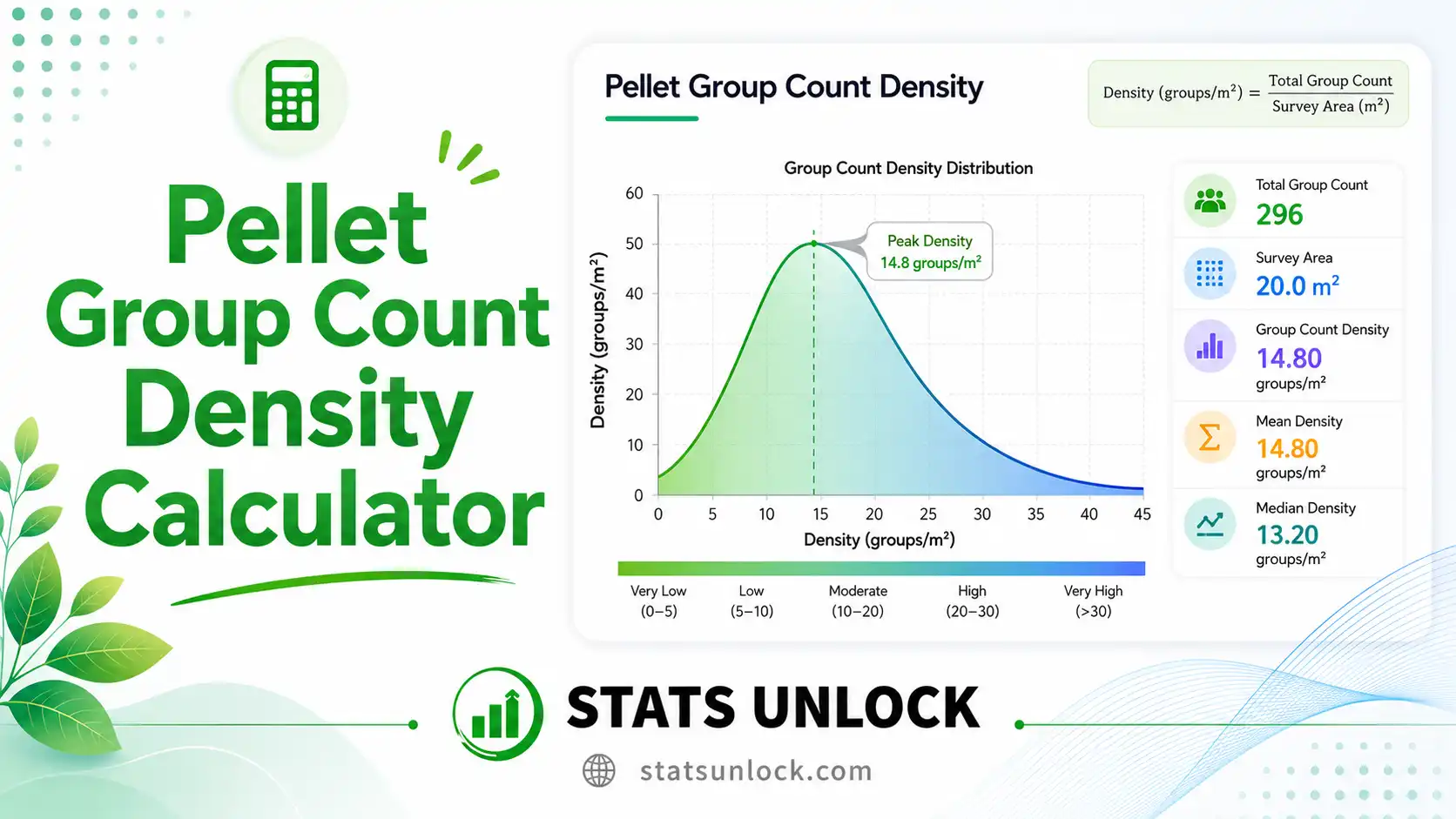
Pellet Group Count Density Calculator
Estimate ungulate density from scat, dung & pellet group counts — a free online indirect wildlife survey method for deer, elk and herbivore population studies.
📊 Density Distribution
📈 Plot Variation
🥧 Density Tiers
📉 Cumulative Effort
📥 Data Input
0 valid values entered
Supports .csv, .txt, .xlsx, .xls — headers auto-detected. Select a numeric column after upload.
| Plot ID | Pellet Count |
|---|
⚙️ Analysis Configuration
📊 Results
Pellet Group Count Density Equation
The formula for pellet group density (D) is:
For animal density: N = D / (R × t)
- D: Pellet group density (groups per unit area, e.g., per hectare)
- Pi: Number of pellet groups counted in plot i
- n: Total number of sample plots surveyed
- A: Area of each sample plot (in same units as D)
- C: Unit-conversion factor (e.g., 10,000 m²/ha)
- N: Animal density (individuals per unit area)
- R: Defaecation rate (pellet groups per animal per day)
- t: Clearance interval (days since plots were cleared)
📋 Full Results Table
| Statistic | Value | Description |
|---|
📊 Pellet Counts by Plot
📈 Distribution Histogram
🥧 Density Tier Breakdown
📉 Cumulative Mean (Stability)
🔬 Plain Language Interpretation
✍️ How to Write Your Results in Research (5 Examples)
🎨 Poster Design Specifications
Typography: Title 72–96 pt (Poppins or Montserrat, bold). Section headers 36–48 pt. Body 24–28 pt minimum. Callouts 60–80 pt.
Colour Palette: Background white or #f8f9fa; primary accent forest green (#16a34a); secondary amber (#d97706); danger muted red (#dc2626). Maximum 3 accent colours.
Standard Sizes: A0 portrait (841 × 1189 mm) for international conferences; 36 × 48 in (914 × 1219 mm) for North American; A1 (594 × 841 mm) for seminars.
Print Resolution: 300 dpi minimum; export as PDF/X-1a for professional print shops.
Software: Canva, PowerPoint, Adobe Illustrator, or Inkscape.
📐 Technical Notes — Formula Derivation, Assumptions & Limitations
Extended Formula Derivation
The standard pellet group count density estimator is derived from the assumption that pellet groups deposited within a plot during a known time interval are proportional to the time-integrated abundance of the source animal. The mean count per plot (x̄ = ∑ Pi / n) is divided by plot area A to give pellet group density. To convert to animal density, the Eberhardt-van Etten formula is applied:
N = (Dpellets) / (R × t)
Where Dpellets is pellet group density (groups/ha), R is the species-specific defaecation rate (typically 12–20 groups per animal per day for cervids), and t is the time in days between plot clearing and recount. Standard error and 95% CI are computed using the sample variance and the t-distribution with n − 1 degrees of freedom.
Key Assumptions
- Pellet groups are deposited randomly across the survey area (no strong avoidance or attraction to plot edges).
- All pellet groups within plots are detected (perfect detection) — corrected via double-observer or removal estimators when violated.
- Defaecation rate (R) is constant and known for the target species and season.
- Decomposition is negligible during the clearance interval, OR a separate decay-rate study is incorporated.
- Pellet groups can be unambiguously identified to species — multi-species areas require careful identification.
Limitations
- Defaecation-rate uncertainty: small errors in R propagate directly into animal density estimates.
- Decay-rate variability: moisture, temperature, and dung-beetle activity affect persistence.
- Habitat-related detection bias: ground vegetation, leaf litter, and soil colour reduce detection.
- Plot size sensitivity: small plots produce zero-inflated counts; large plots are time-consuming.
- Spatial autocorrelation: bedding sites and trails violate independence assumptions.
📌 When to Use This Tool — Decision Guide
Decision Checklist
- You need to estimate ungulate density in habitats where direct observation is difficult (dense forest, montane shrubland).
- Your plot size is standardised across the survey design.
- You have a known clearance interval and either know or can estimate the defaecation rate for your target species.
- You want a low-cost, replicable, indirect index of animal abundance.
- Do NOT use if pellet identification to species is unreliable (mixed deer/livestock landscapes).
- Do NOT use if decomposition rates are highly variable and unmeasured.
- Do NOT use as the sole method for population estimates in management decisions — combine with camera trapping or distance sampling.
Real-World Examples
🦌 Deer Population Surveys
Estimating white-tailed deer density across forest stands of varying management intensity in eastern North America.
🐘 Large Herbivore Monitoring
Indirect surveys of elephant or rhino activity in protected areas where direct counts are impractical.
🦘 Macropod Density Estimation
Scat-based density estimation of kangaroos and wallabies in Australian rangelands and conservation reserves.
🌲 Habitat-Use Comparisons
Comparing deer use across burned vs unburned forest plots, or pre- vs post-restoration treatment areas.
Sampling Design Guidance
- Minimum recommended effort: ≥ 30 plots per habitat type for stable mean estimates.
- Plot size: 4–100 m² rectangles or strips (50 m × 2 m is common); cleared at start of survey period.
- Clearance interval: 30–120 days; shorter for high-decay environments (humid tropics).
- Stratify plots across habitat types to reduce variance.
Related Metrics Decision Tree
Need indirect ungulate density? → Pellet Group Count Density (this tool)
  → Need confirmed species ID? → Add DNA scat genotyping
  → Need temporal activity? → Camera Trap RAI
Need direct counts? → Distance Sampling / Line Transect
Need presence/absence? → Occupancy Modelling
Need community-level diversity? → Shannon-Wiener / Simpson's Index
❓ Frequently Asked Questions
Q1. What is pellet group count density and when should I use it?
Pellet group count density is an indirect wildlife survey method that estimates the number of pellet groups (faecal droppings) per unit area, typically expressed as groups per hectare. It is widely used in deer, elk, and other ungulate research where direct observation is difficult due to dense vegetation or cryptic behaviour.
Use it when you need a low-cost, replicable, non-invasive index of relative abundance — for example, comparing deer use between forest treatment plots, or tracking changes in herbivore activity across seasons.
Q2. What data do I need to calculate pellet group density?
You need three things at minimum: (1) the count of pellet groups recorded in each sample plot, (2) the area of each plot in consistent units (m², ha, or km²), and (3) ideally the time interval since plots were last cleared.
To convert to animal density, you also need a published defaecation rate for your target species (typically 12–20 groups per animal per day for deer). The tool accepts comma-separated counts in the textarea, file upload, or manual table.
Q3. What does a high vs low pellet group density value mean ecologically?
For deer, densities above 500 pellet groups per hectare typically indicate dense populations or heavy site use, often linked to bedding cover or seasonal feeding areas. Moderate values (100–500/ha) reflect typical forest use, while low values (under 50/ha) may indicate marginal habitat, recent disturbance, or low-density populations.
Always interpret in the context of habitat type, season, defaecation rate, and decomposition conditions — raw numbers are not directly comparable across studies without standardisation.
Q4. How does pellet group counting differ from camera trapping?
Pellet counts integrate animal activity over weeks or months and work in dense vegetation where cameras might miss animals. They are inexpensive and require no batteries, but cannot identify individuals or capture activity patterns.
Camera traps give species-specific, time-stamped detections and can record behaviour, but require expensive equipment, theft risk, and detection-distance bias. The two methods are complementary — the strongest deer monitoring programmes use both.
Q5. What are the assumptions and limitations of pellet group density?
Key assumptions: (1) random distribution of pellet groups across the area, (2) complete detection within plots, (3) known and constant defaecation rates, and (4) negligible decomposition during the clearance interval.
Limitations include sensitivity to defaecation-rate uncertainty, decay-rate variability between seasons, habitat-related detection bias, and difficulty identifying pellets to species in mixed-ungulate landscapes.
Q6. How much sampling effort is needed for reliable density estimates?
A practical minimum is 30 plots per habitat type. For low-density populations or habitats with high count variance, 100+ plots may be needed. Use the cumulative-mean stability chart in this tool's results to check whether your sample size is sufficient — a flat tail indicates adequate effort.
Pilot studies are strongly recommended to estimate variance before committing to a full survey design.
Q7. Can I compare pellet group densities between sites or seasons?
Yes, provided sampling effort, plot size, clearance interval, and observer protocols are standardised across all comparisons. Differences in decay rates between seasons (especially monsoon vs dry) must be measured separately and corrected.
For statistical comparison, use bootstrapping, generalised linear mixed models, or non-parametric tests rather than raw mean comparisons. Report effect sizes and 95% confidence intervals.
Q8. How do I report pellet group density in an ecology journal?
Always report: mean density per hectare, 95% confidence interval, standard error, number of plots, plot size, and clearance interval. State the defaecation rate used and its source citation.
See the five reporting templates in the "How to Write Your Results" section above for journal-style, thesis, policy brief, conference abstract, and long-term monitoring formats.
Q9. Can I use this calculator for published research or a university thesis?
This tool is designed for educational use, exploratory analysis, and field-survey planning. For formal publication, verify results using peer-reviewed software such as the R packages distance, pellets, or unmarked, which can handle detection probability and distance-sampling adjustments.
If citing this tool, use: STATS UNLOCK. (2026). Pellet Group Count Density Calculator. Retrieved from https://statsunlock.com/pellet-group-count-density-calculator
Q10. My density value seems unexpectedly high or low — what might have gone wrong?
Common causes: (1) data entry errors (decimal mistakes, mixed units), (2) inclusion of zero-count plots inflating means or skewing variance, (3) mis-identified pellets from non-target species, (4) plots that span multiple habitat types, and (5) incorrect plot size in the configuration field.
Check your raw data in the Manual Entry tab, inspect the histogram and cumulative mean charts for outliers, and verify your plot size and units. Compare against the included sample datasets to verify the tool is behaving correctly.
📖 How to Use This Tool — Step-by-Step Guide
Enter Your Data
Type or paste comma-separated pellet counts (e.g., 52, 48, 55, 61, 47), upload a CSV/Excel file, or use the manual table. The tool accepts 5–500+ plots.
Choose a Sample Dataset
Five built-in USA datasets cover white-tailed deer (Great Smoky Mountains NP), white-tailed deer (Pennsylvania), mule deer (Black Hills NF, South Dakota), elk (Yellowstone), and moose (Voyageurs NP, Minnesota) — pick one to test the workflow.
Configure Settings
Set your plot size (default 100 m²), output units (per hectare is standard), clearance interval in days, defaecation rate (typically 13 for deer), and confidence level (95% is standard).
Run the Analysis
Click the green "Run Analysis" button. The tool computes mean, variance, density per chosen unit, animal density (if defaecation rate provided), and 95% confidence intervals.
Read the Summary Cards
Green = high density (active habitat), amber = moderate (typical use), red = low density (concern or marginal habitat).
Read the Full Results Table
Every statistic is listed: mean, SD, SE, CV, density per ha, animal density, 95% CI bounds, sample size, and total counts.
Examine the Four Charts
Bar chart for plot-level counts, histogram for distribution shape, pie for density tiers, and cumulative mean for sampling adequacy.
Read the Plain-Language Interpretation
Five paragraphs translating numbers into ecological meaning — includes habitat implication and conservation context.
Copy a Reporting Example
Five templates: ecology journal, thesis, policy brief, conference abstract, and long-term monitoring report. Click "Copy" on any.
Export Your Results
Download a plain-text Doc for editing, or a print-ready PDF for archiving and sharing.
🔍 Conclusion
▶ Run the analysis above to generate a personalised conclusion for your dataset.
🔗 Related Tools — Continue Your Ecological Analysis
Once you have estimated pellet group density at your site, the next step is usually to characterise the biodiversity of the wider community using the data you have collected. The free tools below are part of the same Stats Unlock ecology suite — they share the same input format and reporting style, so you can move data between them without reformatting.
Suggested workflow: Use this pellet group count density calculator to estimate herbivore pressure → run the species richness calculator on your survey data to capture community completeness → check community structure with the Shannon-Wiener and Simpson's diversity calculators → finish with the evenness and relative abundance tools to fully characterise your site.
📚 References
The following references support the statistical and ecological methods used in this pellet group count density calculator, covering indirect wildlife survey methods, deer density estimation, and best practices in ecological sampling.
- Eberhardt, L., & Van Etten, R. C. (1956). Evaluation of the pellet group count as a deer census method. Journal of Wildlife Management, 20(1), 70–74. https://doi.org/10.2307/3797250
- Neff, D. J. (1968). The pellet-group count technique for big game trend, census, and distribution: A review. Journal of Wildlife Management, 32(3), 597–614. https://doi.org/10.2307/3798941
- Mayle, B. A., Peace, A. J., & Gill, R. M. A. (1999). How many deer? A field guide to estimating deer population size. Forestry Commission Field Book 18. https://www.forestresearch.gov.uk
- Marques, F. F. C., Buckland, S. T., Goffin, D., Dixon, C. E., Borchers, D. L., Mayle, B. A., & Peace, A. J. (2001). Estimating deer abundance from line transect surveys of dung: Sika deer in southern Scotland. Journal of Applied Ecology, 38(2), 349–363. https://doi.org/10.1046/j.1365-2664.2001.00584.x
- Plumptre, A. J. (2000). Monitoring mammal populations with line transect techniques in African forests. Journal of Applied Ecology, 37(2), 356–368. https://doi.org/10.1046/j.1365-2664.2000.00499.x
- Buckland, S. T., Anderson, D. R., Burnham, K. P., Laake, J. L., Borchers, D. L., & Thomas, L. (2001). Introduction to distance sampling: Estimating abundance of biological populations. Oxford University Press.
- Krebs, C. J. (1999). Ecological methodology (2nd ed.). Benjamin Cummings.
- Fuller, T. K. (1991). Do pellet counts index white-tailed deer numbers and population change? Journal of Wildlife Management, 55(3), 393–396. https://doi.org/10.2307/3808964
- Smart, J. C. R., Ward, A. I., & White, P. C. L. (2004). Monitoring woodland deer populations in the UK: An imprecise science. Mammal Review, 34(1–2), 99–114. https://doi.org/10.1046/j.0305-1838.2003.00026.x
- Acevedo, P., Ferreres, J., Jaroso, R., Durán, M., Escudero, M. A., Marco, J., & Gortázar, C. (2010). Estimating roe deer abundance from pellet group counts in Spain: An assessment of methods suitable for Mediterranean woodlands. Ecological Indicators, 10(6), 1226–1230. https://doi.org/10.1016/j.ecolind.2010.04.006
- Forsyth, D. M., Barker, R. J., Morriss, G., & Scroggie, M. P. (2007). Modeling the relationship between fecal pellet indices and deer density. Journal of Wildlife Management, 71(3), 964–970. https://doi.org/10.2193/2005-695
- Lioy, S., Marsan, A., Balduzzi, A., Wauters, L. A., Martinoli, A., & Preatoni, D. (2015). The strengths and weaknesses of pellet count as a tool for habitat selection studies. Hystrix, 26(2), 123–128. https://doi.org/10.4404/hystrix-26.2-11420
- R Core Team. (2024). R: A language and environment for statistical computing. R Foundation for Statistical Computing. https://www.R-project.org/
- Miller, D. L., Rexstad, E., Thomas, L., Marshall, L., & Laake, J. L. (2019). Distance sampling in R. Journal of Statistical Software, 89(1), 1–28. https://doi.org/10.18637/jss.v089.i01
- Sutherland, W. J. (Ed.). (2006). Ecological census techniques: A handbook (2nd ed.). Cambridge University Press. https://doi.org/10.1017/CBO9780511790508