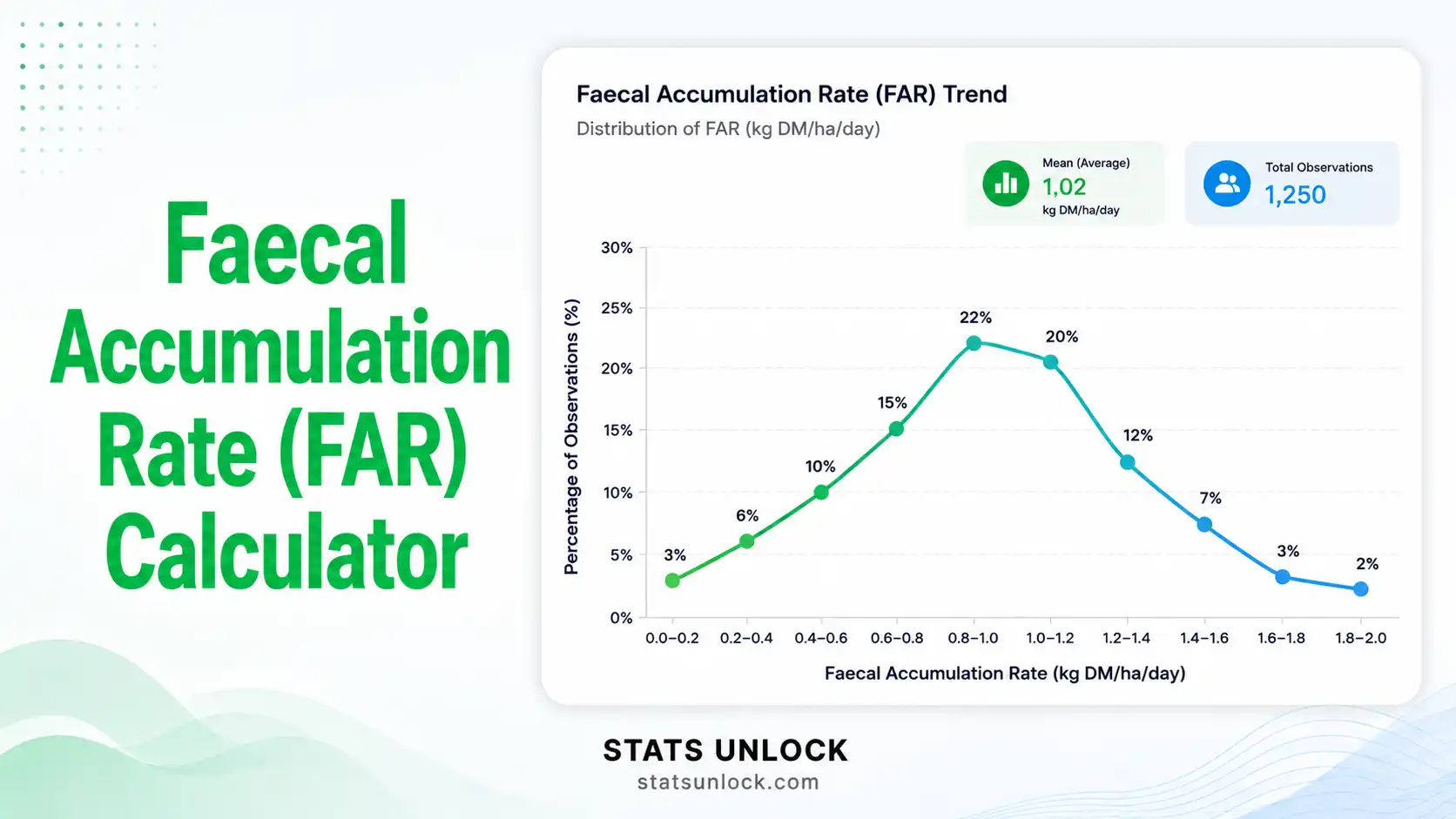
Faecal Accumulation Rate Calculator (FAR) — Free Wildlife Dung Density Tool

📥 Step 1 — Enter Your Pellet Group Counts

Pellet Group Counts (per plot, comma-separated)

Enter one number per plot. Comma- or newline-separated. Each value = pellet groups counted at that plot during the clearance interval.

Use Sample Dataset:

Upload CSV or Excel file:

Supports .csv, .txt, .xlsx, .xls — headers detected automatically.

Add one row per plot. Click "+ Add Plot" to extend.

Plot IDPellet Groups

⚙️ Step 2 — Configure Survey Parameters

Study Area / Site Name

Group Name (editable)

Plot Area (each plot)

Plot Area Unit

Clearance Interval (days)

Defecation Rate (groups/animal/day) Default 25 = white-tailed deer (Rogers 1987)

📊 Results — Summary

Faecal Accumulation Rate Equation

FAR is the count of fresh pellet groups per unit area per unit time:

\[ \text{FAR} = \frac{\sum_{i=1}^{n} P_i}{n \cdot A \cdot t} \]

FAR: Faecal Accumulation Rate (pellet groups · m⁻² · day⁻¹)
P_i: Pellet groups counted at plot i during the clearance interval
n: Total number of cleared plots sampled
A: Area of each plot in square meters (m²)
t: Clearance interval in days (time between clearing and recount)
∑: Sum of pellet group counts across all n plots

Density conversion (Eberhardt & Van Etten 1956):

\[ D = \frac{\text{FAR}}{d} \]

D: Animal density (animals · m⁻²; multiply by 10,000 for animals/ha)
d: Defecation rate (pellet groups · animal⁻¹ · day⁻¹) — species-specific

Statistic	Value	Description

📈 Visualizations

1. Pellet Groups per Plot

2. Distribution Histogram

3. Cumulative Sample Effort

4. FAR & Density (Doughnut)

📥 Export Your Report

📖 Plain Language Interpretation

Subsection 1 — Detailed Interpretation Results

Subsection 2 — How to Write Your Results in Research

▶ Five ready-to-use reporting templates auto-filled with your computed values. Use the 📋 Copy button on each card.

🪧 Research Poster Panel

Print-ready A0/A1 poster layout — auto-filled with your latest results. Copy whole panel or rebuild in Canva/PowerPoint.

📌 Poster Design Specifications (typography, palette, sizes, software)

Sizes: A0 portrait (841 × 1189 mm) for full conferences; A1 portrait (594 × 841 mm) for institutional showcases.
Title typography: 90–110 pt bold sans-serif (DM Sans, Lato, or Montserrat); subtitle 40–48 pt regular.
Body typography: 24–28 pt for primary text; section headers 36–42 pt bold; references 9–10 pt.
Color palette: Forest green primary (#3aab6d), bright accent (#52c98a), mint background (#f0faf4), dark green-grey text (#1a3528). Keep ≤ 4 colors to avoid visual clutter.
Print resolution: Export at 300 DPI minimum; embed all fonts; convert to PDF/X-1a for commercial print.
Recommended software: Canva (templates), PowerPoint (set custom slide size), Adobe InDesign (professional), Inkscape (free vector).
Reading distance: Title legible at 6–8 feet; body text legible at 3–4 feet.
QR code: Place bottom-right, ≥ 4 cm × 4 cm, link to dataset DOI or preprint.

🌿 Detailed Conclusion

📌 When to Use the FAR Method (Decision Checklist)

Use FAR when:

Target species is a large herbivore producing distinct pellet groups (deer, elk, moose, pronghorn, bison)
Animals are too cryptic, nocturnal, or low-density for reliable direct counts
Survey area is closed or fenced (no immigration/emigration during interval)
A standardized clearance interval (14–60 days) is logistically feasible
A defecation rate from peer-reviewed literature exists for the focal species

Do NOT use FAR when:

Pellet groups cannot be reliably distinguished from other species' droppings
Ground cover is too dense or disturbed for complete plot clearance
Clearance interval exceeds local pellet decay time (very wet or hot climates)
Species defecation rate is unknown (use Standing Crop method instead)

Real-World USA Examples:

Pennsylvania Game Commission — annual deer browse and density surveys in mixed hardwood state forests
Yellowstone elk monitoring — winter range FAR plots in Lamar Valley meadows
Texas Parks & Wildlife — white-tailed deer density estimation in Hill Country chaparral
Maine IFW moose population estimates — boreal forest pellet group surveys post-snowmelt

Sampling Design Guidance:

Use ≥ 30 plots per stratum (60+ for heterogeneous habitat). Stratify by habitat type, slope, and distance to forage. Random or systematic placement; clearance interval 30–60 days in temperate climates; revisit within 2 days of target endpoint to minimize decay loss.

Related Metrics — Decision Tree:

Need herbivore density without direct counts?  → Faecal Accumulation Rate (FAR)
  → Plots can be cleared and revisited?         → FAR (this tool)
  → Single visit only, no clearance possible?   → Standing Crop pellet method (apply decay rate)
Need to detect carnivores or omnivores?         → Camera trap RAI / scat genetics
Need habitat use intensity (not density)?       → Encounter Rate per km / track surveys
Need community-level diversity?                 → Shannon-Wiener / Simpson's Diversity Index
Need occupancy with imperfect detection?        → Single-season occupancy model (unmarked R package)

📚 How to Use This Tool — 10-Step Guide

Enter Your Data — Paste comma-separated pellet counts (e.g., 52, 48, 55, 61, 47), upload a CSV/Excel from your field data sheet, or use the manual table. Worked example: a Pennsylvania researcher cleared 30 forest plots and counted 52, 48, 55, 61, 47 pellet groups at the first 5 plots after a 30-day interval.
Choose a Sample Dataset — Select from 5 USA datasets: PA white-tailed deer, Yellowstone elk, Colorado mule deer, Maine moose, or Texas low-density deer. Sample 1 loads on first render.
Configure Survey Parameters — Enter your plot area (default 100 m²), clearance interval in days (default 30), and defecation rate (default 25 groups/animal/day for white-tailed deer). The Group Name field is fully editable — change it to "Elk" or "Moose" as needed.
Run the Analysis — Click "Calculate Faecal Accumulation Rate." The tool computes mean FAR, total pellets, density (animals/m² and animals/km²), and 95% confidence interval.
Read the Summary Cards — Color coding: green = high herbivore activity (FAR ≥ 0.005), amber = moderate (0.001–0.005), blue = low (< 0.001). Cards show total groups, mean FAR, density, and CV (variability).
Read the Full Results Table — Every row carries a description: total plots, mean and SD of pellet counts, FAR with units, density per unit area, defecation rate used. Confirm your inputs are correct.
Examine the Four Visualizations — (1) Bar chart per plot identifies hotspots; (2) histogram shows whether counts are skewed (Poisson-like) or uniform; (3) cumulative effort plot reveals if 30 plots was enough; (4) doughnut shows FAR vs density on a single dial.
Read the Detailed Interpretation — Five auto-filled paragraphs translate the FAR value into a management statement; use the journal/thesis/policy/abstract/monitoring report templates in the Plain Language section.
Copy a Reporting Example — Each of the 5 example cards has a Copy button. Paste the journal-style version into your manuscript or the policy version into a USDA/state agency report.
Export Your Results — Use Download Doc for a plain-text report (paste into Word) or Download PDF for a print-ready A4 report with all 8 sections.

❓ Frequently Asked Questions

Q1. What is the Faecal Accumulation Rate (FAR) and when should I use it?

FAR (Faecal Accumulation Rate) is the number of fresh pellet groups deposited per unit area per unit time, measured by clearing field plots of all old dung and counting newly deposited groups after a known interval. It is the standard indirect-survey method for cryptic large herbivores — used widely in USA wildlife agencies for white-tailed deer, mule deer, elk, moose, and pronghorn population assessment.

Use FAR when direct counts (drive surveys, aerial census) are impractical due to dense cover, nocturnal behavior, or low density. The Pennsylvania Game Commission, Wisconsin DNR, and the National Park Service all use FAR as a routine population index.

Q2. What data do I need to calculate FAR?

Three required inputs: (1) pellet group counts at each cleared plot, (2) plot area (typically 1–100 m²), and (3) clearance interval in days. One optional input — the species defecation rate (groups/animal/day) — is needed to convert FAR to animal density. Standard USA values: 25 groups/day for white-tailed deer (Rogers 1987), 14 groups/day for elk (Neff 1968), 13 groups/day for moose.

The Paste tab works best for short field data sheets; the Upload tab handles full CSV/Excel exports from FieldMaps, Survey123, or QField.

Q3. What does a high vs low FAR value mean ecologically?

For white-tailed deer in productive eastern US forests, typical FAR values range from 0.001 to 0.01 pellet groups · m⁻² · day⁻¹. Values above 0.005 indicate high local density (≥ 20 deer/km²) — often associated with browse damage and oak regeneration failure. Values below 0.001 indicate low density (< 5 deer/km²) — typical of the western US arid range.

For elk, FAR > 0.003 in Yellowstone winter range signals locally concentrated herds. Always compare to baselines from your state wildlife agency before drawing conclusions.

Q4. How does FAR differ from the Standing Crop pellet count method?

FAR (accumulation method) clears plots first, then revisits after a known interval — only fresh pellet groups are counted. Standing Crop counts ALL pellets present without clearing, then divides by an estimated decay rate. FAR is more accurate (no decay assumption) but requires two visits per plot. Standing Crop is faster but errors compound when decay rate is poorly known.

USA-specific guidance: use FAR east of the 100th meridian (where wet conditions accelerate decay); Standing Crop is acceptable in arid western states with peer-reviewed decay rates.

Q5. What are the assumptions and limitations of FAR?

Key assumptions: (a) plots are completely cleared before the interval; (b) clearance interval is shorter than typical decay time; (c) defecation rate is constant by sex, age, and season; (d) plots are randomly placed; (e) animals do not avoid (or prefer) cleared plots. Limitations: cannot identify individuals, cannot detect short-term population changes, sensitive to climatic variation in pellet decay, and ineffective for omnivores or species with overlapping pellet morphology (e.g., elk vs cattle in mixed-use landscapes).

Q6. How much sampling effort do I need for FAR to be reliable?

Minimum thresholds: 30 plots for white-tailed deer in homogeneous habitat; 60–100 plots for elk or moose in heterogeneous landscapes. Use a clearance interval of 30–60 days in temperate USA climates and 14–30 days in humid southeastern states (Florida, Louisiana) where decay is rapid. Increase plot count when CV of pellet counts > 100% or when stratifying across multiple habitat types.

Q7. Can I compare FAR values between sites or seasons?

Yes — provided plot size, clearance interval, observer protocol, and seasonal timing are standardized. Use bootstrapped 95% CI or two-sample t-tests for between-site comparison. Avoid pooling FAR collected with different clearance intervals without first converting to common units (groups · m⁻² · day⁻¹). Cross-state comparisons (e.g., PA vs WI) are valid only when methodology is identical.

Q8. How do I report FAR in a wildlife journal or USDA report?

Required elements: mean FAR with units (groups · m⁻² · day⁻¹), 95% CI, n (plot count), plot size (m²), clearance interval (days), total pellet groups counted, defecation rate value and citation, and resulting density estimate. Cite the original method paper (Eberhardt & Van Etten 1956 or Neff 1968). See Subsection 2 above for five ready-to-paste reporting templates covering Journal of Wildlife Management style, dissertation style, USDA policy brief style, conference abstract style, and long-term monitoring style.

Q9. Can I use this calculator for published research or a university thesis?

Yes — formulas implemented here follow Eberhardt & Van Etten (1956) and Neff (1968), the canonical FAR references. For peer-reviewed publication, cross-check with R packages (distance, unmarked) and report this tool in your methods. Site citation: STATS UNLOCK. (2026). Faecal Accumulation Rate (FAR) Calculator. Retrieved from https://statsunlock.com/faecal-accumulation-rate-calculator.

Q10. My FAR value seems unexpectedly high or low — what might have gone wrong?

Common errors: (1) plot area unit mix-up — m² vs hectares shifts FAR by 10,000× (most common); (2) clearance interval entered incorrectly (e.g., 0 instead of 30); (3) incomplete plot clearance — old pellets misclassified as new; (4) decay during long intervals deflates FAR (use shorter intervals in wet climates); (5) miscount of pellet groups (one defecation = one group, not single pellets — a deer pellet group has 30–80 pellets). Cross-check by loading Sample Dataset 1 — if expected output matches, your raw data is the issue.

📚 References

The following references support the methods used in this Faecal Accumulation Rate (FAR) calculator, covering indirect wildlife survey, pellet group count methodology, and best practices in large herbivore density estimation in North America.

Eberhardt, L., & Van Etten, R. C. (1956). Evaluation of the pellet group count as a deer census method. Journal of Wildlife Management, 20(1), 70–74. https://doi.org/10.2307/3797250
Neff, D. J. (1968). The pellet-group count technique for big game trend, census, and distribution: A review. Journal of Wildlife Management, 32(3), 597–614. https://doi.org/10.2307/3798941
Rogers, L. L. (1987). Seasonal changes in defecation rates of free-ranging white-tailed deer. Journal of Wildlife Management, 51(2), 330–333. https://doi.org/10.2307/3801010
Fuller, T. K. (1991). Do pellet counts index white-tailed deer numbers and population change? Journal of Wildlife Management, 55(3), 393–396. https://doi.org/10.2307/3808966
Marques, F. F. C., Buckland, S. T., Goffin, D., Dixon, C. E., Borchers, D. L., Mayle, B. A., & Peace, A. J. (2001). Estimating deer abundance from line transect surveys of dung: Sika deer in southern Scotland. Journal of Applied Ecology, 38(2), 349–363. https://doi.org/10.1046/j.1365-2664.2001.00584.x
Forsyth, D. M., Barker, R. J., Morriss, G., & Scroggie, M. P. (2007). Modeling the relationship between fecal pellet indices and deer density. Journal of Wildlife Management, 71(3), 964–970. https://doi.org/10.2193/2005-695
Smart, J. C. R., Ward, A. I., & White, P. C. L. (2004). Monitoring woodland deer populations in the UK: An imprecise science. Mammal Review, 34(1–2), 99–114. https://doi.org/10.1046/j.0305-1838.2003.00026.x
Krebs, C. J. (1999). Ecological methodology (2nd ed.). Benjamin Cummings.
Buckland, S. T., Anderson, D. R., Burnham, K. P., Laake, J. L., Borchers, D. L., & Thomas, L. (2001). Introduction to distance sampling: Estimating abundance of biological populations. Oxford University Press.
Acevedo, P., Ferreres, J., Jaroso, R., Durán, M., Escudero, M. A., Marco, J., & Gortázar, C. (2010). Estimating roe deer abundance for management purposes: A direct comparison of two methods. European Journal of Wildlife Research, 56(2), 199–208. https://doi.org/10.1007/s10344-009-0301-4
Pennsylvania Game Commission. (2023). Deer management annual report. Bureau of Wildlife Management. https://www.pgc.pa.gov
Fiske, I., & Chandler, R. (2011). unmarked: An R package for fitting hierarchical models of wildlife occurrence and abundance. Journal of Statistical Software, 43(10), 1–23. https://doi.org/10.18637/jss.v043.i10
R Core Team. (2024). R: A language and environment for statistical computing. R Foundation for Statistical Computing. https://www.R-project.org/
Sawyer, H., Nielson, R. M., Lindzey, F. G., Keith, L., Powell, J. H., & Abraham, A. A. (2007). Habitat selection of Rocky Mountain elk in a nonforested environment. Journal of Wildlife Management, 71(3), 868–874. https://doi.org/10.2193/2006-094
U.S. National Park Service. (2022). Long-term ecological monitoring protocols: Ungulate populations. NPS Inventory & Monitoring Program. https://www.nps.gov/im/