

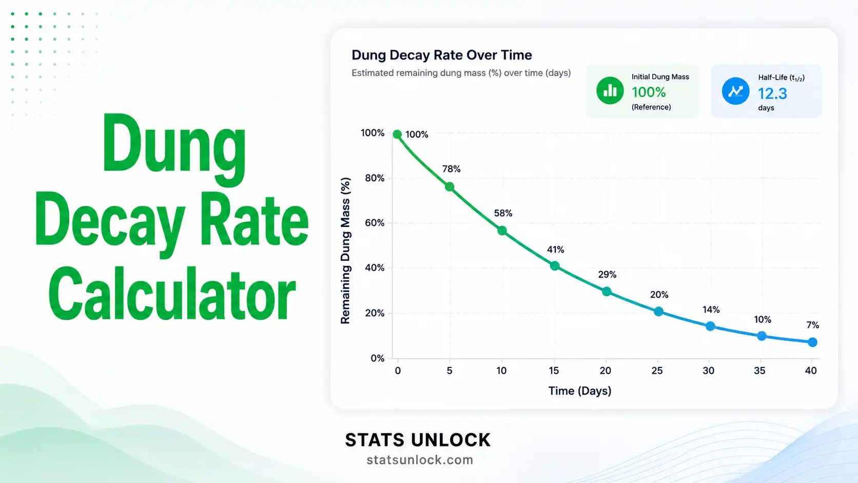

Dung Decay Rate Calculator
Estimate the dung and scat decay constant (k), half-life (t½), and persistence times for wildlife dung-count surveys — for deer, elephants, ungulates, and carnivores.
📋 1. Enter Your Dung / Scat Cohort Data
Mark a cohort of fresh dung piles on day 0 and revisit at successive time intervals. Enter the number of intact piles still detectable at each visit.
Day 0 is the day dung piles were marked. Use the actual elapsed days at each revisit.
Comma-separated counts (default). One value per visit, in the same order as the days above.
Supports .csv, .txt, .xlsx, .xls — headers detected automatically.
| Day Since Deposition | Intact Piles |
|---|
⚙️ 2. Survey Context & Parameters
Optional metadata — populates results, reporting templates, poster, and exported reports. Set N₀ and defecation rate before calculating.
Total piles marked on day 0 — used to compute survival proportion S(t) = N(t)/N₀.
Used for indicative density estimation via FSC × k ÷ defecation rate.
🧭 7. When to Use This Tool
- You marked a cohort of fresh dung piles and revisited them at known intervals
- You want a defensible decay constant k and half-life for a dung-count density estimate
- You need a season- and habitat-specific decay rate (Laing et al. 2003 framework)
- You are running indirect, non-invasive wildlife surveys for deer, elk, elephant, ungulates, or carnivores
- Do NOT use a single decay rate across multiple seasons — fit one per season
- Do NOT use if your cohort had < 30 marked piles — precision will be poor (Marques et al. 2001)
- Do NOT use exponential decay if you suspect rapid early loss + slow tail — fit a Weibull or two-stage model instead
Real-world USA examples
🦌 White-tailed deer dung decay — Pennsylvania state forests
Cohort of 80 fresh dung piles marked in October. Revisits at 14, 28, 56, 84, and 112 days yielded k ≈ 0.018 /day; half-life ≈ 38 days. Used for state-wide population indices.
🦌 Elk dung decay — Yellowstone National Park
Winter cohort decay typically k ≈ 0.005–0.008 /day (slow under snow); summer cohort k ≈ 0.025–0.035 /day. Demonstrates the necessity of season-specific decay correction.
🐘 Elephant dung decay — Zoo Knoxville & comparative African studies
Tropical decay k ≈ 0.020–0.040 /day; half-life 17–35 days. Used in Distance-sampling FSC estimates of African elephant density.
🐺 Grey wolf scat persistence — Yellowstone & Idaho
Scat decay k ≈ 0.012–0.025 /day; faster on roads, slower in forest interior. Critical for non-invasive genetic monitoring sampling intervals.
Sampling-design guidance
Mark ≥ 60 piles per cohort for ~10% precision on k (Laing et al. 2003); revisit at 4–6 intervals spanning at least 2 half-lives. Replicate cohorts in space (≥ 3 plots) and across seasons. Always pair the decay study with a matched-clearance dung-count survey for density estimation.
🛠️ 8. How to Use This Tool — Step-by-Step
- Mark a fresh cohort. On day 0, locate and individually flag (numbered pin / GPS waypoint / photograph) at least 60 fresh dung piles in your study area. Record N₀.
- Plan revisits. Choose 4–6 revisit days spanning roughly 2 expected half-lives — for deer this is typically 14, 28, 42, 56, 70, 84 days.
- Score persistence. At each visit, count how many marked piles are still intact (definitions in Marques et al. 2001 — recognisable as the original deposit).
- Choose a sample dataset from the drop-down to see how the tool works, or paste your own counts (comma-separated) in the textarea. Default placeholder:
52, 48, 55, 61, 47, ... - Configure analysis. Enter the study area name, taxon, habitat, season, initial cohort size N₀, and (optionally) the species-specific defecation rate.
- Click Calculate. The tool fits an exponential decay model and returns k, t½, R², and projected disappearance times.
- Read the four plots. Decay curve (observed vs fitted), linearised log-survival, per-interval rate, and persistence forecast.
- Interpret. Read the auto-filled paragraphs in §3 — they explain what your k means ecologically and which decay tier (slow/moderate/fast) it falls into.
- Copy a reporting example. Five styles are provided plus a research poster panel — pick the one matching your audience.
- Export your results. Click 📋 Doc for a plain-text report or 🖨️ PDF for a formatted print-ready PDF including all eight sections.
❓ 9. Frequently Asked Questions
What is dung decay rate?
Dung decay rate is the proportion of dung, scat, or feces piles that disappear from the ground per unit of time, usually expressed as a decay constant (k, /day) or a half-life (t½, days). It is a critical correction factor in dung-count and faecal standing-crop wildlife surveys.
How is the dung decay constant (k) calculated?
The decay constant is fitted from an exponential decay model N(t) = N₀ · e−kt. In practice we transform to ln(N(t)/N₀) = −kt and fit a linear regression — the negative slope is k. This tool uses ordinary least-squares on log-transformed survival proportions.
What is dung half-life?
Half-life (t½) is the number of days for half the original cohort to disappear. It equals ln(2)/k. A k of 0.02 /day corresponds to a half-life of about 35 days.
Why is decay rate critical for dung count surveys?
Dung-count density estimates require a decay correction. Faecal standing crop (FSC) gives D = FSC × k / defecation rate. Without an accurate k, density estimates are biased — a high decay rate overestimates density and a low decay rate underestimates it.
How many cohorts do I need to estimate decay rate reliably?
At least 30 marked piles per cohort and 4–6 monitoring intervals are recommended (Marques et al. 2001). Laing et al. (2003) recommend 60–100 piles for 10% precision on k.
Does decay rate vary by season?
Yes — substantially. Decay is faster in warm wet conditions due to dung beetles, fungi, and microbial activity, and slower in cold dry conditions. Always estimate decay locally and seasonally; never copy values from another study.
Can I use one decay rate for the whole year?
No. Combining seasonal decay rates biases density estimates. Use season-specific decay rates and the FSC matched-clearance method described by Buckland et al. (2010).
What units does this calculator use?
Counts of intact dung piles per cohort across days. The model returns k in /day, half-life in days, and projected 50%/75%/95%/99% disappearance times.
Does this tool work for elephant dung, deer dung, and carnivore scat?
Yes — the exponential decay model is taxon-agnostic. It works equally for elephant boli, deer dung, ungulate dung, and carnivore scat. Just choose the appropriate species and habitat.
What R package equivalents does this implement?
It mirrors the dung-decay logic in the dssd, Distance, and pellet R packages — exponential decay fit by log-linear regression. For more advanced fits (mixed-effects, Weibull, or zero-inflated models) the R packages give finer control.
🔗 10. Related StatsUnlock Tools & Guides
Explore other free wildlife and ecology calculators on StatsUnlock.com.
📚 11. References
The following references support the dung decay rate calculator and its use in wildlife dung-count surveys, faecal standing crop methodology, and non-invasive density estimation.
- Laing, S. E., Buckland, S. T., Burn, R. W., Lambie, D., & Amphlett, A. (2003). Dung and nest surveys: estimating decay rates. Journal of Applied Ecology, 40(6), 1102–1111. doi.org/10.1111/j.1365-2664.2003.00861.x
- Hiby, L., & Lovell, P. (1991). Dung surveys versus line transects: an experimental comparison of two methods for estimating elephant numbers. In African Wildlife: Research and Management (pp. 73–87). ICSU Press.
- Plumptre, A. J., & Harris, S. (1995). Estimating the biomass of large mammalian herbivores in a tropical montane forest: a method of faecal counting that avoids assuming a 'steady state' system. Journal of Applied Ecology, 32(1), 111–120. doi.org/10.2307/2404420
- Marques, F. F. C., Buckland, S. T., Goffin, D., Dixon, C. E., Borchers, D. L., Mayle, B. A., & Peace, A. J. (2001). Estimating deer abundance from line transect surveys of dung: sika deer in southern Scotland. Journal of Applied Ecology, 38(2), 349–363. doi.org/10.1046/j.1365-2664.2001.00584.x
- Buckland, S. T., Plumptre, A. J., Thomas, L., & Rexstad, E. A. (2010). Design and analysis of line transect surveys for primates. International Journal of Primatology, 31(5), 833–847. doi.org/10.1007/s10764-010-9431-5
- Neff, D. J. (1968). The pellet-group count technique for big game trend, census, and distribution: a review. Journal of Wildlife Management, 32(3), 597–614. doi.org/10.2307/3798941
- Putman, R. J. (1984). Facts from faeces. Mammal Review, 14(2), 79–97. doi.org/10.1111/j.1365-2907.1984.tb00341.x
- Wallmo, O. C., Jackson, A. W., Hailey, T. L., & Carlisle, R. L. (1962). Influence of rain on the count of deer pellet groups. Journal of Wildlife Management, 26(1), 50–55. doi.org/10.2307/3798167
- Barnes, R. F. W., & Jensen, K. L. (1987). How to count elephants in forests. IUCN African Elephant & Rhino Specialist Group Technical Bulletin, 1, 1–6.
- Massei, G., Bacon, P., & Genov, P. V. (1998). Fallow deer and wild boar pellet group disappearance in a Mediterranean area. Journal of Wildlife Management, 62(3), 1086–1094. doi.org/10.2307/3802561
- Nchanji, A. C., & Plumptre, A. J. (2001). Seasonality in elephant dung decay and implications for censusing and population monitoring in south-western Cameroon. African Journal of Ecology, 39(1), 24–32. doi.org/10.1046/j.1365-2028.2001.00264.x
- Lunt, N., Bowkett, A. E., & Plowman, A. B. (2007). Implications of assumption violation in density estimates of antelope from dung-pile counts. African Journal of Ecology, 45(3), 481–487. doi.org/10.1111/j.1365-2028.2007.00768.x
- Krebs, C. J. (1999). Ecological methodology (2nd ed.). Benjamin Cummings.
- R Core Team. (2024). R: A language and environment for statistical computing. R Foundation for Statistical Computing. www.R-project.org
- Miller, D. L., Rexstad, E., Thomas, L., Marshall, L., & Laake, J. L. (2019). Distance Sampling in R. Journal of Statistical Software, 89(1), 1–28. doi.org/10.18637/jss.v089.i01