Scat Diet Composition Calculator
Quantify carnivore diet from scat samples — frequency of occurrence (%FO), percent occurrence (%PO), and prey item composition with publication-ready output.
📥 Step 1 — Enter Your Scat Diet Data
Comma-separated (default). One value per prey item. Example: 52, 48, 55, 61, 47 means 52 scats contained Prey 1, 48 contained Prey 2, etc.
Headers detected automatically. After upload, choose which column contains the prey item names and which contains the scat counts.
⚙️ Step 2 — Configure Analysis
If left blank, calculated from your data assuming each value is "scats containing item".
Items below this %FO are flagged as minor / incidental prey.
📊 Step 3 — Summary Results
Scat Diet Composition Equations
Two complementary metrics describe diet composition from scat:
- %FOi: Frequency of occurrence of prey item i (% of scats containing item i)
- %POi: Percent occurrence of prey item i (share of all prey hits)
- ni: Number of scats containing prey item i
- N: Total number of scats analysed
- ∑ nj: Sum of all prey occurrences across every prey item
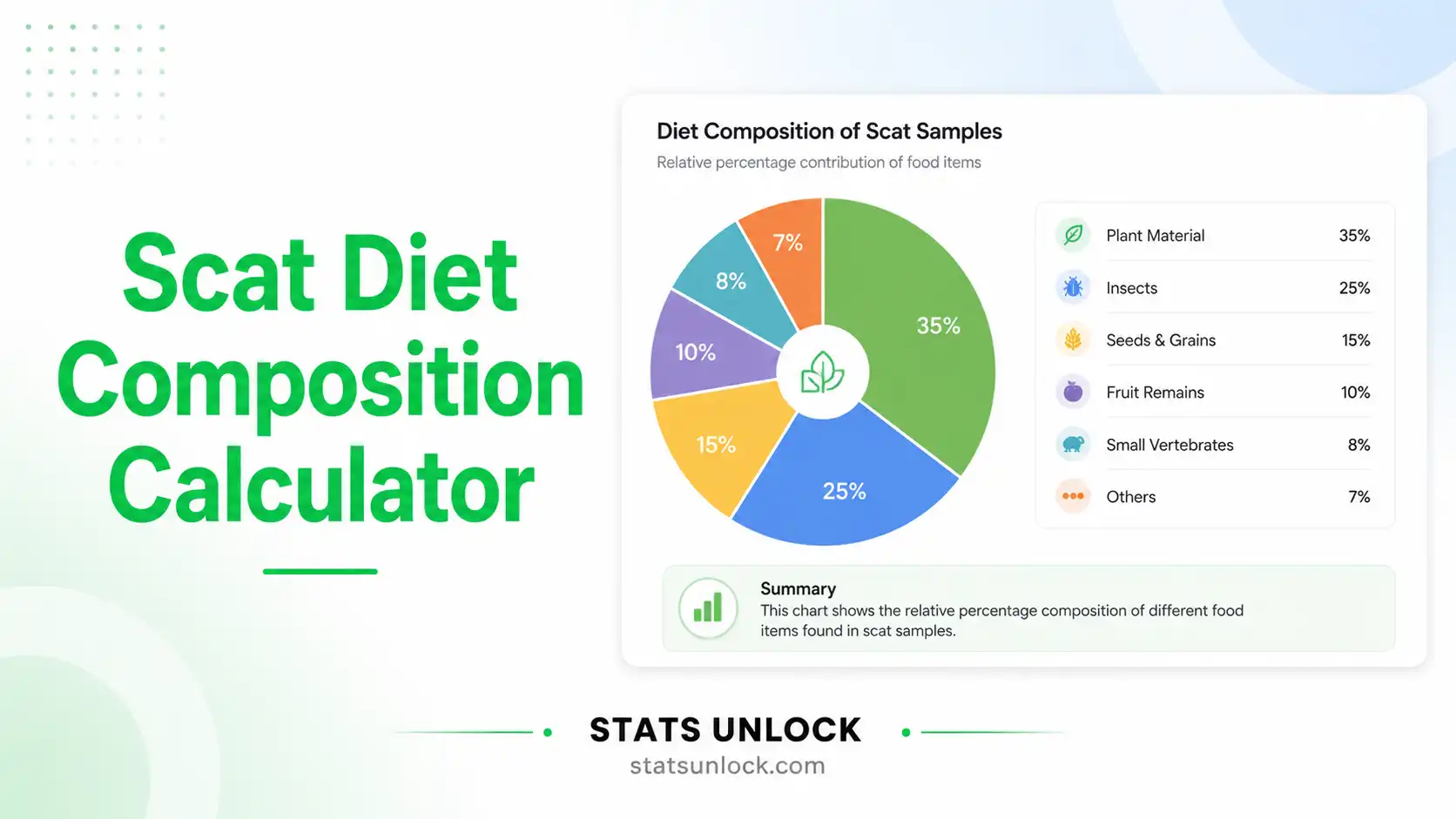
- Note: %FO can sum to > 100% (one scat may contain multiple prey items); %PO sums to 100%.
📋 Full Diet Composition Table
| # | Prey Item | Scats with Item (n) | %FO | %PO | Diet Tier |
|---|
🏆 Top Prey Spotlight
The single most important prey item identified in the diet — a hero callout you can drop straight into a presentation or report.
🎯 Diet Tier Breakdown
Prey items grouped by their dietary importance class. PRIMARY items are dominant (≥50% of scats); SECONDARY items are common; INCIDENTAL items are rare or scavenged.
📐 Advanced Diet Diversity Metrics
Standard ecological diversity indices computed on %PO. Useful for cross-study comparison and reviewer requests.
📖 What do these metrics mean?
- Shannon-Wiener H' — combines richness and evenness; higher = more diverse diet. Typical range 0–3.5.
- Simpson's D — probability that two randomly chosen prey hits are the same species; lower = more diverse.
- Inverse Simpson (1/D) — effective number of equally-common prey items.
- Pielou's J' — evenness on 0–1 scale; 1 = perfectly even, < 0.5 = highly skewed diet.
- Berger-Parker d — proportion of the most dominant prey item; complements diet skew.
- Margalef's DMg — richness corrected for sample size.
- Hill N₁ & N₂ — effective species numbers (exp(H') and 1/D respectively).
- Levins' B (standardised BA) — niche breadth; BA > 0.6 = generalist, < 0.4 = specialist.
⚖️ Diet Niche Breadth (Levins' Standardised B)
Where this carnivore sits on the specialist–generalist continuum. Standardised Levins' B (BA) ranges from 0 (perfect specialist on one prey) to 1 (perfect generalist).
📈 Statistical Confidence & Significance
Wilson 95% confidence interval for the dominant prey's %FO, plus a chi-square goodness-of-fit test against a uniform-diet null hypothesis.
95% Confidence Interval — Dominant Prey %FO
Chi-Square Test — Uniform Diet Null Hypothesis
🗂️ Quick Reference Summary
All key numbers in one glance — handy for citing in a manuscript or pasting into a results table.
📌 At-a-Glance
📤 Export Results
🔬 Detailed Interpretation Results
📝 How to Write Your Results in Research
Five ready-to-use reporting templates plus a research poster panel — auto-filled with your computed values.
🔍 Detailed Conclusion
📊 What Was Found
🌱 Ecological Significance
🌿 Conservation & Management Implications
🔭 Next Steps & Methodological Guidance
🎯 Take-Home Synthesis
🧮 Technical Notes — Formulas, Assumptions & Limitations
Extended Formula Derivation
The two core diet composition metrics share the same numerator (ni) but differ in their denominator. Frequency of occurrence (%FO) uses the total number of scat samples (N) as the denominator, treating each scat as a Bernoulli trial that either contains or does not contain prey item i. Percent occurrence (%PO) uses the sum of all prey hits across all items (∑nj), so each prey item's share is normalised to total prey occurrences rather than to total scats.
Because a single scat can contain multiple prey items, the sum of %FO across all prey items often exceeds 100%, while the sum of %PO is always exactly 100%. This is why both metrics should be reported together — %FO answers "how many scats contained this prey?" while %PO answers "what fraction of the diet does this prey item make up?"
Assumptions
- Scats are correctly identified to the predator species (use genetic confirmation when sympatric carnivores overlap).
- Prey remains are correctly identified from hair, bone, feather, scale, or seed fragments.
- Differential digestion among prey is not corrected for in raw %FO and %PO — small/soft prey may be under-detected.
- Sampling effort is sufficient to reach the asymptote of a cumulative prey-item curve (typically ≥ 50–100 scats).
- Each scat is treated as an independent observation; collect across spatial and temporal replicates to avoid pseudo-replication.
Limitations
- %FO and %PO do not estimate biomass consumed — large prey items contribute disproportionately to nutrition but may appear in fewer scats.
- Highly digestible prey (e.g., small mammals consumed whole) may be over-represented relative to large prey.
- Hair-only identification cannot distinguish scavenging from predation.
- Insect remains may be over-represented because of their indigestible chitinous exoskeletons.
- For biomass-corrected estimates, apply correction factors from Floyd, Mech & Jordan (1978) or Ackerman, Lindzey & Hemker (1984).
🎯 When to Use This Tool — Decision Checklist
Use this calculator when:
- ✓ You have collected scats from a known predator species and identified prey remains in each sample.
- ✓ You want to summarise diet composition as %FO and %PO for a manuscript, thesis, or report.
- ✓ You want to compare diet between seasons, sites, or sex/age classes within a species.
- ✓ Your sampling effort is at or near the cumulative prey-item asymptote (typically ≥ 50 scats).
Do NOT use this calculator when:
- ✗ Sample sizes are very small (< 30 scats) — confidence intervals become uninformative.
- ✗ You need biomass estimates — apply published correction factors first.
- ✗ You want to test diet selectivity — combine with prey-availability data and use Manly's α or Ivlev's E.
- ✗ Predator species identification is uncertain — confirm scat origin with genetic methods.
Real-world USA examples:
- Coyote diet in Yellowstone (Wyoming) — quantifying ungulate vs small-mammal contributions across summer and winter.
- Bobcat scat analysis in Texas Hill Country — assessing the role of cottontail and small rodents during drought years.
- Gray wolf diet on Isle Royale (Michigan) — long-term moose dependency and beaver subsidy.
- Mountain lion scat in Idaho — evaluating mule deer reliance versus elk during winter.
Sampling design guidance:
- Collect 50–100 scats per season per site.
- Plot a cumulative prey-item curve to confirm sample size adequacy.
- Stratify by season and habitat type to capture diet shifts.
- Store scats frozen or in alcohol; process under sterile conditions.
📚 How to Use This Tool — Step-by-Step Guide
- Enter your data — Paste scat counts (e.g.,
52, 48, 55, 61, 47) into the textarea, or use Column Entry for labelled prey items, or upload a CSV/Excel file. - Choose a sample dataset — Five USA carnivore datasets are pre-loaded for testing.
- Set the study area — Optional but recommended; populates reporting templates and the PDF cover.
- Edit the group name — Default is "Coyote (Canis latrans)"; change to your study species.
- Enter total scats (N) — Required for %FO calculation; defaults to the dataset's reported N.
- Configure thresholds — Choose diet-diversity threshold and minor-prey cutoff.
- Click "Run Scat Diet Analysis" — Computes %FO and %PO for every prey item, with diet tier classification.
- Read the four colourful charts — %FO bar, %PO donut, cumulative contribution, and diet profile scatter.
- Read the diet composition table — Each row shows raw count, %FO, %PO, and diet tier (primary/secondary/incidental).
- Read the detailed interpretation and conclusion — Plain-language paragraphs with study area substitution.
- Copy a reporting example — Five styles (ecology journal, thesis, plain-language, conference abstract, monitoring) plus a research poster panel.
- Export — Download Doc (.txt) or PDF for archiving.
❓ Frequently Asked Questions
What is scat diet composition analysis?
What is %FO and how is it calculated?
What is %PO and how does it differ from %FO?
Should I report %FO, %PO, or both?
How many scat samples are needed for a reliable diet study?
How do I distinguish predation from scavenging in scat?
Can I use this for omnivores like black bears?
How are biomass estimates calculated and why aren't they shown here?
What software can I use to compare two scat datasets statistically?
Is this tool free to use for graduate research?
📚 References
The following references support the methods used in this scat diet composition calculator, covering frequency of occurrence, percent occurrence, and best practices in carnivore feeding ecology across USA wildlife studies.
- Floyd, T. J., Mech, L. D., & Jordan, P. A. (1978). Relating wolf scat content to prey consumed. Journal of Wildlife Management, 42(3), 528–532. https://doi.org/10.2307/3800814
- Ackerman, B. B., Lindzey, F. G., & Hemker, T. P. (1984). Cougar food habits in southern Utah. Journal of Wildlife Management, 48(1), 147–155. https://doi.org/10.2307/3808462
- Klare, U., Kamler, J. F., & Macdonald, D. W. (2011). A comparison and critique of different scat-analysis methods for determining carnivore diet. Mammal Review, 41(4), 294–312. https://doi.org/10.1111/j.1365-2907.2011.00183.x
- Litvaitis, J. A. (2000). Investigating food habits of terrestrial vertebrates. In L. Boitani & T. K. Fuller (Eds.), Research techniques in animal ecology (pp. 165–190). Columbia University Press. Columbia University Press
- Reynolds, J. C., & Aebischer, N. J. (1991). Comparison and quantification of carnivore diet by faecal analysis: a critique, with recommendations, based on a study of the fox Vulpes vulpes. Mammal Review, 21(3), 97–122. https://doi.org/10.1111/j.1365-2907.1991.tb00113.x
- Ciucci, P., Boitani, L., Pelliccioni, E. R., Rocco, M., & Guy, I. (1996). A comparison of scat-analysis methods to assess the diet of the wolf Canis lupus. Wildlife Biology, 2(1), 37–48. https://doi.org/10.2981/wlb.1996.006
- Trites, A. W., & Joy, R. (2005). Dietary analysis from fecal samples: How many scats are enough? Journal of Mammalogy, 86(4), 704–712. https://doi.org/10.1644/1545-1542(2005)086[0704:DAFFSH]2.0.CO;2
- Bartnick, T. D., Van Deelen, T. R., Quigley, H. B., & Craighead, D. (2013). Variation in cougar (Puma concolor) predation habits during wolf (Canis lupus) recovery in the southern Greater Yellowstone Ecosystem. Canadian Journal of Zoology, 91(2), 82–93. https://doi.org/10.1139/cjz-2012-0147
- Vanak, A. T., & Gompper, M. E. (2009). Dietary niche separation between sympatric free-ranging domestic dogs and Indian foxes in central India. Journal of Mammalogy, 90(5), 1058–1065. https://doi.org/10.1644/09-MAMM-A-107.1
- Spaulding, R., Krausman, P. R., & Ballard, W. B. (2000). Observer bias and analysis of gray wolf diets from scats. Wildlife Society Bulletin, 28(4), 947–950. JSTOR 3783847
- Mukherjee, S., Goyal, S. P., & Chellam, R. (1994). Standardisation of scat analysis techniques for leopard (Panthera pardus) in Gir National Park, western India. Mammalia, 58(1), 139–143. https://doi.org/10.1515/mamm.1994.58.1.139
- Hayward, M. W., Henschel, P., O'Brien, J., Hofmeyr, M., Balme, G., & Kerley, G. I. H. (2006). Prey preferences of the leopard (Panthera pardus). Journal of Zoology, 270(2), 298–313. https://doi.org/10.1111/j.1469-7998.2006.00139.x
- R Core Team. (2024). R: A language and environment for statistical computing. R Foundation for Statistical Computing. https://www.R-project.org/
- Oksanen, J., Simpson, G. L., Blanchet, F. G., et al. (2022). vegan: Community ecology package. R package version 2.6-4. https://CRAN.R-project.org/package=vegan
- Stats Unlock. (2026). Scat Diet Composition Calculator. https://statsunlock.com/scat-diet-composition-calculator