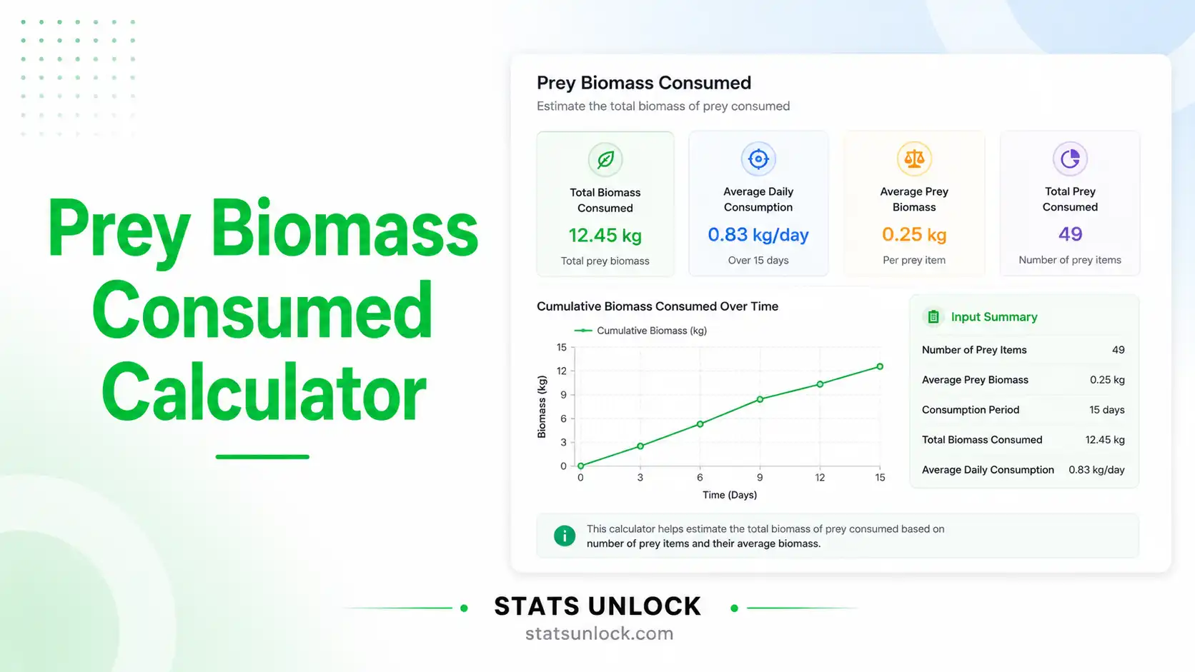
Prey Biomass Consumed Calculator
Estimate the total prey biomass consumed by predators in a study area — a core metric for carnivore ecology, food web flow, and predator-prey conservation planning.
📥 Data Input
Optional. Auto-filled into all reports and the research poster.
Predator group: e.g., wolf pack, cougar territory, grizzly bear family group.
Number of predators in the population.
Period over which kills are summed (default = 365 days).
Number of kill events per prey species.
Average body mass per individual prey (kilograms).
Fraction of carcass actually consumed (typical 0.65–0.90).
All examples use real US wildlife scenarios.
Use the Column Entry mode in the Paste / Type tab for full row-based editing.
🔬 Technical Notes
Extended Formula Derivation & Equivalent Forms
The total prey biomass consumed (B) by a predator population over a defined interval is the sum, across all prey species, of the product of kill frequency, body mass, and the consumption coefficient (the carcass-utilisation efficiency).
General form:
Per-predator daily intake (kg/predator/day):
Annualised, per-predator (kg/predator/year):
Equivalent kill-rate form (when consumption coefficients are unknown, set c = 1.0 to estimate gross prey production removed):
Assumptions
- All kills attributable to the focal predator group are detected (or detection probability is corrected for).
- Mean body mass mᵢ reflects the actual mass of prey killed (large predators frequently kill above-mean individuals — adjust if biased).
- The consumption coefficient cᵢ accounts for scavenger loss; for solitary felids 0.65–0.80 is typical; for social canids 0.80–0.95.
- Kill counts are independent and not double-counted between cluster events.
- Time window T is biologically meaningful (e.g., a full annual cycle for migratory prey).
Limitations
- Detection bias: GPS-cluster-derived kill rates miss small prey; snow-tracking misses non-snow seasons.
- Scavenger loss: Wolves, bears, and corvids may consume substantial portions of carcasses; the coefficient c only approximates this.
- Sample window: Predator kill rates vary seasonally — annualising a 90-day winter sample inflates summer estimates.
- Energetics not biomass: Biomass is not equivalent to energy; fat content varies enormously between summer and winter prey.
- Compensatory predation: Some prey killed would have died anyway (winter starvation); the metric does not separate additive from compensatory mortality.
🎯 When to Use This Tool
Decision Checklist
- You have kill records (count of kills per prey species) from GPS-cluster, snow-tracking, scat, or kill-site surveys
- You know — or can estimate — mean body mass per prey species (kg)
- You want to estimate annual or per-predator prey requirements for management
- You need a publication-ready biomass estimate for a peer-reviewed wildlife journal
- You want to test whether the prey base is sufficient to support a predator recovery population
- Do NOT use if your kill detection probability is unknown — apply a correction factor first (Knopff et al. 2010)
- Do NOT use for energetic intake studies — use field metabolic rate models (Carbone & Gittleman 2002) instead
- Do NOT use if scavenger loss is significant and you have no c estimate — report gross biomass only
Real-World Examples (USA Wildlife)
- Yellowstone Wolf-Elk System: Smith et al. estimated that a 10-wolf pack consumes ~88,000 kg of elk biomass per year, equivalent to ~22 elk per wolf annually.
- Yellowstone Cougars: Solo cougars consume 30–55 kg of ungulate biomass per week; a 100-cougar landscape population removes > 600 t of mule deer and elk per year.
- Florida Panther Recovery: Each panther consumes ~1,250 kg of prey biomass per year, dominated by white-tailed deer (~75%) and feral hogs (~20%).
- Greater Yellowstone Grizzlies: Adult grizzlies consume 700–1,800 kg of prey biomass per year, but ungulate biomass is only ~25–40% of total intake (vegetation and insects fill the rest).
Sampling Design Guidance
- Detect ≥ 30 kills per predator group per season for stable estimates (Sand et al. 2008).
- For GPS-collared predators: cluster-search ≥ 80% of clusters > 4 hours.
- Use scat-based DNA + biomass conversion for cryptic predators (Mumma et al. 2014).
- Replicate across ≥ 2 seasons to capture seasonal variation in prey selection.
- Pair with prey density estimates (DistANCE sampling, line transects) to compute predation rate.
Related Metrics — Decision Tree
📖 How to Use This Tool
Step-by-Step Walkthrough (10 Steps)
- Enter your data — paste kill counts, body masses, and consumption coefficients in the three textareas, or use Column Entry mode for row-by-row input. Example: 52 elk, 48 mule deer, 18 bison killed by a 10-wolf pack in 365 days.
- Choose a sample dataset — five US wildlife scenarios are pre-loaded (Yellowstone wolf, Yellowstone cougar, GYE grizzly, Northern Rockies wolf, Florida panther).
- Configure the analysis — set your predator count (P), the time period (T, in days), and an optional study area name. The group name (e.g., "Lamar Canyon Pack") is editable.
- Click Run Analysis — the tool computes total biomass B, per-predator daily intake I, annual per-predator intake A, and per-species contributions.
- Read the summary cards — green = abundant biomass intake (typical of intact prey base); amber = moderate; red = below the IUCN minimum prey-availability threshold.
- Read the full results table — total biomass, per-predator daily/annual intake, and a breakdown of every prey species' contribution.
- Examine all four charts — biomass per species, proportional contribution, kills vs biomass, and a cumulative biomass curve.
- Read the detailed interpretation — five paragraphs explaining what was found, the magnitude, ecosystem context, practical relevance, and limitations.
- Copy a reporting example — use Ecology Journal style for peer review, Plain-Language for managers, and Conference Abstract for posters.
- Export your results — Word/Doc for a written report, PDF for printing or archiving. Both files are auto-named with your study area.
❓ Frequently Asked Questions
What is prey biomass consumed?
Prey biomass consumed is the total weight (kg or metric tons) of prey eaten by a predator population over a defined period. It is a core metric in carnivore ecology because it directly links predator demography to ecosystem-level energy flow.
How is the formula B = Σ(n × m × c) different from kill rate?
Kill rate measures the frequency of kills (kills/predator/day). Biomass consumed measures the mass actually eaten, accounting for prey size differences and scavenger loss via the consumption coefficient c.
What is a typical consumption coefficient (c)?
For solitary large felids (cougars, leopards): c ≈ 0.65–0.80. For social canids (wolves): c ≈ 0.80–0.95. For grizzlies on ungulates: c ≈ 0.70–0.90. Use c = 1.0 to report gross biomass produced (no scavenger correction).
How do I get kill counts (n)?
Three main methods: (1) GPS-cluster investigation of collared predators; (2) snow-tracking with backtracking to kill sites; (3) DNA-based scat analysis combined with prey-mass conversion factors.
Can I use this for fish or invertebrate predators?
Yes — the formula is taxon-agnostic. Use kg-equivalent biomass for fish prey (wet weight) and dry-mass for invertebrate prey. Just be consistent across species.
How does this compare to predator energy requirements?
Convert biomass to energy with prey-specific conversion factors (typically 5,500–8,500 kJ/kg fresh weight for ungulates). Compare to field metabolic rate (FMR) from Carbone & Gittleman (2002): FMR ≈ 4.91 W₀.86 (W = predator body mass kg).
What if I only have kill counts but not body mass?
Use published mean body mass for adult animals from your region (e.g., Yellowstone elk ≈ 320 kg, mule deer ≈ 90 kg). Cite the body-mass source. Alternatively, use the gross biomass form B = Σ(n × m) without c.
Why is this useful for IUCN assessments?
The IUCN guideline of ~50 ungulates per predator (Karanth et al. 2004) translates directly to a biomass requirement. If your computed biomass falls below ~ 1,500 kg/predator/year for a tiger or 800 kg/predator/year for a cougar, the prey base is potentially insufficient.
How do I incorporate uncertainty into the estimate?
Bootstrap the kill counts (1,000 iterations), resample mean body masses from a normal distribution with the SE from a body-mass dataset, and report the 95% percentile interval. Some authors propagate uncertainty in c using Beta distributions.
How do I cite this tool?
Cite as: STATS UNLOCK Prey Biomass Consumed Calculator (2026). https://statsunlock.com/. In Methods, also cite Vucetich et al. (2011) or Hayward et al. (2006) for the underlying biomass framework.
🔍 Detailed Conclusion
▶ Run the analysis above to generate a personalised conclusion for your dataset.
📚 References
The following references support the wildlife ecology methods used in this prey biomass consumed calculator, covering predator-prey dynamics, carnivore energetics, and best practices in kill-site investigation and biomass estimation.
- Vucetich, J. A., Hebblewhite, M., Smith, D. W., & Peterson, R. O. (2011). Predicting prey population dynamics from kill rate, predation rate and predator-prey ratios in three wolf-ungulate systems. Journal of Animal Ecology, 80(6), 1236–1245. https://doi.org/10.1111/j.1365-2656.2011.01855.x
- Hayward, M. W., O'Brien, J., & Kerley, G. I. H. (2006). Carrying capacity of large African predators: Predictions and tests. Biological Conservation, 139(1–2), 219–229. https://doi.org/10.1016/j.biocon.2007.06.018
- Carbone, C., & Gittleman, J. L. (2002). A common rule for the scaling of carnivore density. Science, 295(5563), 2273–2276. https://doi.org/10.1126/science.1067994
- Knopff, K. H., Knopff, A. A., Warren, M. B., & Boyce, M. S. (2009). Evaluating global positioning system telemetry techniques for estimating cougar predation parameters. Journal of Wildlife Management, 73(4), 586–597. https://doi.org/10.2193/2008-294
- Sand, H., Wabakken, P., Zimmermann, B., Johansson, Ö., Pedersen, H. C., & Liberg, O. (2008). Summer kill rates and predation pattern in a wolf-moose system. Oecologia, 156(1), 53–64. https://doi.org/10.1007/s00442-008-0969-2
- Smith, D. W., Drummer, T. D., Murphy, K. M., Guernsey, D. S., & Evans, S. B. (2004). Winter prey selection and estimation of wolf kill rates in Yellowstone National Park, 1995–2000. Journal of Wildlife Management, 68(1), 153–166. https://doi.org/10.2193/0022-541X(2004)068
- Karanth, K. U., Nichols, J. D., Kumar, N. S., Link, W. A., & Hines, J. E. (2004). Tigers and their prey: Predicting carnivore densities from prey abundance. PNAS, 101(14), 4854–4858. https://doi.org/10.1073/pnas.0306210101
- Metz, M. C., Smith, D. W., Vucetich, J. A., Stahler, D. R., & Peterson, R. O. (2012). Seasonal patterns of predation for gray wolves in the multi-prey system of Yellowstone National Park. Journal of Animal Ecology, 81(3), 553–563. https://doi.org/10.1111/j.1365-2656.2011.01945.x
- Mumma, M. A., Soulliere, C. E., Mahoney, S. P., & Waits, L. P. (2014). Enhanced understanding of predator-prey relationships using molecular methods to identify predator species, individual, and sex. Molecular Ecology Resources, 14(1), 100–108. https://doi.org/10.1111/1755-0998.12153
- Ruth, T. K., Buotte, P. C., & Hornocker, M. G. (2019). Yellowstone cougars: Ecology before and during wolf restoration. University Press of Colorado. https://upcolorado.com/utah-state-university-press/item/3494-yellowstone-cougars
- Hebblewhite, M., White, C. A., Nietvelt, C. G., McKenzie, J. A., Hurd, T. E., Fryxell, J. M., Bayley, S. E., & Paquet, P. C. (2005). Human activity mediates a trophic cascade caused by wolves. Ecology, 86(8), 2135–2144. https://doi.org/10.1890/04-1269
- Pierce, B. M., Bleich, V. C., & Bowyer, R. T. (2000). Selection of mule deer by mountain lions and coyotes: Effects of hunting style, body size, and reproductive status. Journal of Mammalogy, 81(2), 462–472. https://doi.org/10.1644/1545-1542(2000)081
- Mech, L. D., & Peterson, R. O. (2003). Wolf-prey relations. In L. D. Mech & L. Boitani (Eds.), Wolves: Behavior, ecology, and conservation (pp. 131–160). University of Chicago Press. https://press.uchicago.edu/ucp/books/book/chicago/W/bo3641392.html
- R Core Team. (2024). R: A language and environment for statistical computing. R Foundation for Statistical Computing. https://www.R-project.org/
- U.S. Fish & Wildlife Service. (2024). Yellowstone wolf monitoring annual report. National Park Service. https://www.nps.gov/yell/learn/nature/wolf-reports.htm