

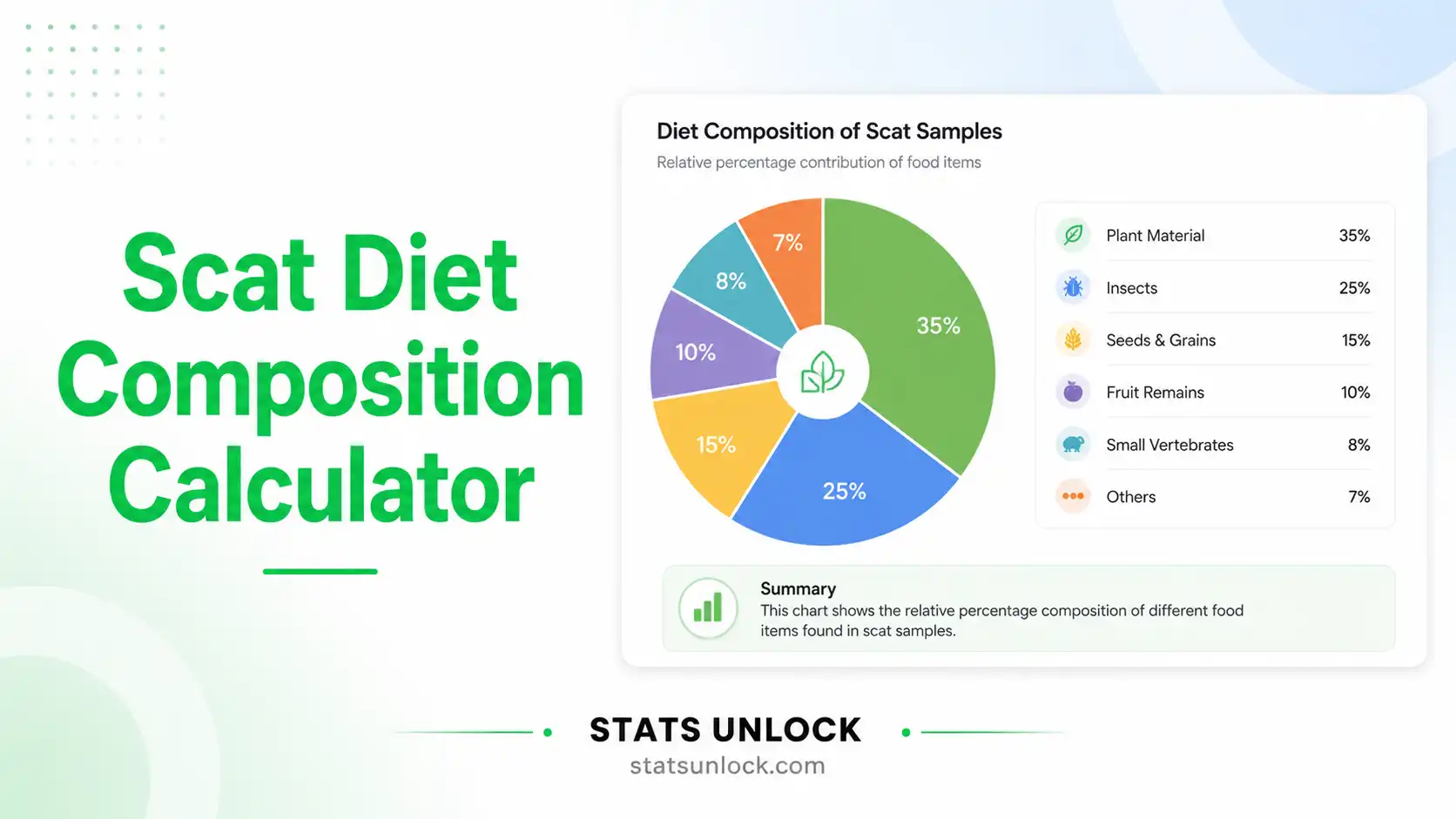

Scat Diet Composition Calculator
Analyze fecal samples to quantify predator diet — compute Frequency of Occurrence, Percentage Occurrence, Index of Relative Importance, Levins' Niche Breadth, and Shannon Dietary Diversity from scat data.
Enter the total scat samples collected (N). Each count above = number of scats in which that item appeared.
Supports .csv, .txt, .xlsx, .xls. Headers detected automatically. Select one column for Food Item / Prey Group Names and one for Occurrence Counts.
Enter food items and their occurrence counts directly in the table below.
| # | Food Item / Prey Group | Occurrence Count | Remove |
|---|
📐 Formulas Used in This Analysis
- ni = number of scats containing food item i
- N = total number of scat samples analyzed
- FO% = Frequency of Occurrence percentage
- %O = Percentage Occurrence (relative to all FO% values)
- IRI = Index of Relative Importance (Pinkas et al., 1971)
- pi = %Oi / 100 (proportional occurrence)
- n = total number of food categories
- BA = Standardized Levins' Niche Breadth (0–1)
- H' = Shannon Dietary Diversity Index (nats)
| Rank | Food Item / Prey | Count (ni) | FO% | %O | IRI | IRI% | IRI Contribution |
|---|
🥧 Diet Composition (IRI%)
📊 Frequency of Occurrence (%)
📈 IRI by Food Item
🔵 Percentage Occurrence (%O)
🔍 1. Overall Diet Summary & Dietary Breadth
🥩 2. Primary & Secondary Prey Items (IRI Analysis)
📉 3. Frequency of Occurrence Interpretation
🌿 4. Ecological Significance & Dietary Strategy
⚠️ 5. Sampling Adequacy & Methodological Caveats
Journal writing conventions
Use passive voice. Report N, number of food items, IRI% for top items, FO% range, and niche breadth BA. Cite Pinkas et al. (1971) for IRI and Levins (1968) for B. Include a results table as a separate supplementary item. Round to two decimal places.
Thesis writing conventions
Write in a formal tone with full methodological justification. Include subsections on data collection, prey identification protocols, and analytical methods. Report all metrics with 95% CI where available. Discuss sampling adequacy using species accumulation curves or rarefaction.
Policy writing conventions
Avoid technical jargon. Use bullet points. Emphasize conservation implications — prey availability, human-wildlife conflict potential, and habitat management actions. Translate FO% and IRI% into plain percentages ("this species eats X about Y% of the time").
Abstract writing conventions
Limit to 250–300 words. State objective, methods (N, species, region), 3–4 key numerical results, and the main conclusion. Include keywords line. Follow the conference template for structured vs. unstructured abstract format.
Monitoring report conventions
Include seasonal or annual comparisons if data span multiple periods. Highlight changes in primary prey FO% or IRI% over time. Use tables for cross-year comparison. Follow the standardized reporting template of your monitoring program (e.g., LTER, WPA annual report format).
Introduction
Run the analysis above to generate poster content.
Methods
___
Key Results
Discussion
___
Conclusions
___
📐 Poster Design Specifications
Recommended sizes: A0 (841×1189mm), A1 (594×841mm), or 48×36 inch landscape.
Typography: Title: 72–96pt bold. Section headers: 36–48pt. Body: 24–28pt. Caption: 18–20pt.
Color palette: Deep forest green (#1b5e20) for headers; soft mint (#e8f5e9) for backgrounds; amber (#e65100) for highlights; white for main body panels.
Software: Adobe Illustrator, Canva, Microsoft PowerPoint (portrait, A0 custom size), or InkScape.
Print resolution: 300 DPI minimum for all figures. Export charts from this tool at 2× resolution for print quality.
Charts: Include all four plots from the Visualization section. Place pie chart (IRI%) centrally; surround with FO% bar chart and IRI bar chart. Captions required for all figures.
🔬 Technical Notes & Methodological Assumptions
IRI Formula: This calculator uses the Pinkas et al. (1971) formulation: IRI = (%O + FO%) × FO%. Some publications use volume (%V) instead of or in addition to %O. When %V data are available, replace %O with %V for a more complete IRI estimate.
Frequency of Occurrence: FO% is the most commonly used and least biased estimator of prey importance in scat analysis. It does not require volume estimation, reducing observer bias from differential digestion rates of hard prey parts.
Bias from Differential Digestibility: Hard-bodied prey (insects, reptiles) and items with indigestible remains (hair, seeds) may be over-represented relative to soft-bodied prey (fish, fruit flesh). Correction factors (e.g., Laundré 1981) should be applied where published digestion coefficients are available.
Levins' Niche Breadth: B is sensitive to sample size. BA (standardized) corrects for the number of categories and is more suitable for comparisons across studies or seasons.
Shannon Dietary Diversity (H'): Calculated using natural logarithm (nats). Some studies use log₂ (bits) or log₁₀. Specify the base in your methods section.
Minimum Sample Size: Estimates stabilize at N ≥ 30 per season. Use species (item) accumulation curves to assess sampling adequacy before reporting results.
Assumptions: Each scat represents one feeding event. Individual animal identity is unknown unless genetic sexing/individual identification is performed. Scats collected at the same site on the same day may not be independent.
- ✔ You are studying carnivore, omnivore, or herbivore food habits through non-invasive sampling
- ✔ You need to quantify prey preferences or seasonal dietary shifts without direct observation
- ✔ You want to compare diet overlap between species or between seasons/habitats
- ✔ You have at least 30 scat samples per study period and have identified food item remains
- ✔ You need publication-ready metrics: FO%, %O, IRI, Levins' B, Shannon H'
- ✗ You only have fewer than 10 scat samples — results will be unreliable
- ✗ Scats cannot be confidently assigned to the target species — use camera trap or GPS collar confirmation
- ✗ You need biomass or caloric intake estimates — use prey biomass consumed analysis instead
- ✔ You are writing up a Master's or PhD chapter on predator ecology, human-wildlife conflict, or conservation management
- ✔ You need to support wildlife management decisions (e.g., livestock depredation mitigation, prey base management)
- Collect and identify scat samples. For each scat, record all food item remains present (hair, bones, seeds, insect exoskeleton, feathers, etc.). Identify to the lowest taxonomic level possible.
- List your food categories. Decide on the grouping level — species, genus, order, or functional group (e.g., "Small Mammals," "Fruits," "Insects"). Enter these as Group Names.
- Count occurrences per food item. For each food category, count the number of scat samples in which that item was detected (presence/absence per scat). This is your occurrence count (ni).
- Enter total scat samples (N). Input the total number of scats analyzed in the study period — not the sum of occurrences (items can co-occur in a single scat).
- Enter your data. Use Free Text (comma-separated), Column Entry (label + value rows), File Upload (.csv/.xlsx), or the Manual Table. A sample sloth bear dataset is pre-loaded for reference.
- Check the sample size. Ensure N ≥ 30 (ideally ≥ 50) per season for reliable FO% estimates. Warn if N is small (tool flags this automatically).
- Click "Run Diet Composition Analysis." The tool computes FO%, %O, IRI, IRI%, Levins' B, BA, and Shannon H' instantly.
- Review the results table. Items are ranked by IRI%. The top-ranked item is the most important in the diet. IRI bar widths reflect relative importance visually.
- Examine the four charts. Pie chart = overall diet proportions (IRI%). Bar charts = FO% by item, IRI by item, and %O by item.
- Use the writing templates. Copy the auto-generated journal, thesis, policy, abstract, or poster text directly into your manuscript or report. Download the full report as .txt or print to PDF.
This scat diet composition calculator and its ecological metrics are based on foundational and recent peer-reviewed references in wildlife diet analysis, predator ecology, and scatological methods.
- Pinkas, L., Oliphant, M. S., & Iverson, I. L. K. (1971). Food habits of albacore, bluefin tuna, and bonito in California waters. California Department of Fish and Game, Fishery Bulletin, 152, 1–105. doi:10.1577/1548-8659
- Levins, R. (1968). Evolution in Changing Environments. Princeton University Press. doi:10.1515/9780691209418
- Shannon, C. E., & Weaver, W. (1949). The Mathematical Theory of Communication. University of Illinois Press. doi
- Putman, R. J. (1984). Facts from faeces. Mammal Review, 14(2), 79–97. doi:10.1111/j.1365-2907.1984.tb00341.x
- Floyd, T. J., Mech, L. D., & Jordan, P. A. (1978). Relating wolf scat content to prey consumed. Journal of Wildlife Management, 42(3), 528–532. doi:10.2307/3800795
- Jedrzejewski, W., & Jedrzejewska, B. (1992). Foraging and diet of the red fox Vulpes vulpes in relation to variable food resources in Bialowieza National Park, Poland. Ecography, 15(2), 212–220. doi:10.1111/j.1600-0587.1992.tb00024.x
- Egbert, A. L., & Stokes, A. W. (1976). The social behaviour of brown bears on an Alaskan salmon stream. Bears: Their Biology and Management, 3, 41–56. doi
- Lockie, J. D. (1959). The estimation of the food of foxes. Journal of Wildlife Management, 23(2), 224–227. doi:10.2307/3797567
- Reid, N., Lundy, M. G., & Montgomery, W. I. (2010). Minimum convex polygon home ranges and diet of the red squirrel. Mammal Review, 40(2), 1–18. doi:10.1111/j.1365-2907.2009.00154.x
- Lanszki, J., & Heltai, M. (2002). Feeding habits of golden jackal and red fox in south-western Hungary. Mammalian Biology, 67(3), 129–136. doi:10.1078/1616-5047-00021
- Klare, U., Kamler, J. F., & Macdonald, D. W. (2011). A comparison and critique of different scat-analysis methods for determining carnivore diet. Mammal Review, 41(4), 294–312. doi:10.1111/j.1365-2907.2011.00183.x
- Ramakrishnan, U., Coss, R. G., & Pelkey, N. W. (1999). Tiger decline caused by the reduction of large ungulate prey. Biological Conservation, 89(2), 113–120. doi:10.1016/S0006-3207(98)00153-X
- Karanth, K. U., & Sunquist, M. E. (1995). Prey selection by tiger, leopard and dhole in tropical forests. Journal of Animal Ecology, 64(4), 439–450. doi:10.2307/5647
- Gittleman, J. L. (1985). Carnivore body size: ecological and taxonomic correlates. Oecologia, 67(4), 540–554. doi:10.1007/BF00790026
- Morisita, M. (1959). Measuring the dispersion of individuals and analysis of the distributional patterns. Memoirs of the Faculty of Science, Kyushu University. Series E (Biology), 2, 215–235. doi