

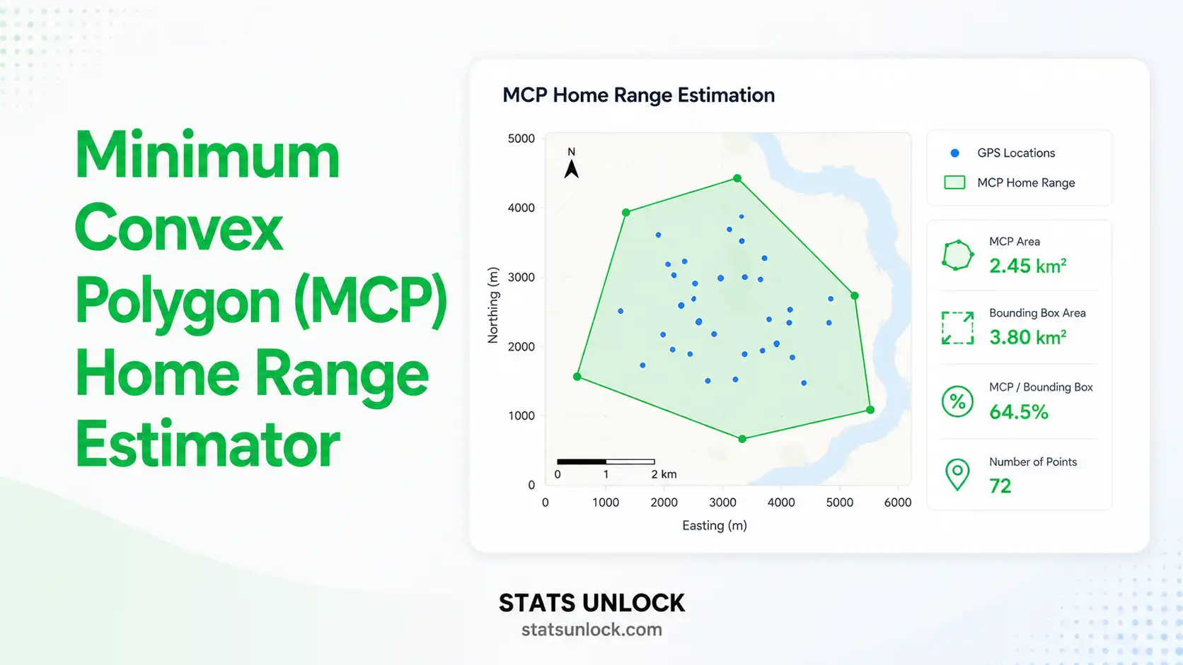

Minimum Convex Polygon
(MCP) Home Range Estimator
Calculate animal home range area from GPS telemetry data using the Minimum Convex Polygon method. Enter coordinates, get instant results with charts and publication-ready output.
GPS Location Data Input
0 latitude values
0 longitude values
0 rows entered
Analysis Configuration
MCP Home Range Results
The Minimum Convex Polygon home range is computed in three steps:
- A: Home range area (m², converted to ha / km² / acres)
- S: Set of GPS fix locations (after outlier trimming for <100% MCP)
- conv(S): Convex hull — smallest convex polygon enclosing S
- xᵢ, yᵢ: Projected Cartesian coordinates of hull vertex i (metres, local tangent plane)
- R: Mean Earth radius = 6,371,000 m (WGS84 spherical)
- For %MCP < 100%: Points beyond the centroid-distance percentile cutoff are excluded before hull computation
Detailed Results Table
| Statistic | Value | Description |
|---|
Visualizations (4 Charts)
Detailed Interpretation Results
▶ Run the analysis above to see detailed interpretation results.
How to Write Your Results in Research
▶ Run the analysis above to auto-fill all six reporting examples.
Conclusion
▶ Run the analysis above to generate a detailed conclusion.
🔬 Technical Notes — MCP Algorithm, Assumptions & Limitations
Algorithm: Graham Scan Convex Hull
This tool uses the Graham scan algorithm (O(n log n)) to compute the convex hull of projected GPS fixes. Points are first converted from WGS84 decimal degrees to local Cartesian coordinates (metres) using the Haversine formula, centred on the centroid of the point cloud. The Shoelace (Surveyor's) formula then gives the polygon area. This approach is accurate within ±0.5% for study areas up to ~100 km across.
Outlier Trimming for % MCP
For <100% MCP (e.g., 95% MCP), points are sorted by their Euclidean distance from the centroid in projected space and the most distant (100 − MCP)% are excluded before computing the hull. This reduces the influence of occasional exploratory forays that inflate the home range estimate.
Assumptions
- Coordinates are in WGS84 decimal degrees
- GPS fixes are representative of actual animal locations
- Movement is not limited by geographic barriers within the polygon
- Fixes are reasonably independent (no severe autocorrelation correction applied)
Limitations
- MCP overestimates actual area used — treats all space within polygon as habitat
- Area estimate is sensitive to sample size (n < 30 is unreliable)
- Does not identify core areas or probability of use (use KDE for this)
- Does not correct for GPS fix autocorrelation (use AKDE for correction)
- Projection accuracy decreases for study areas >200 km across
When to Use MCP vs. KDE
Use MCP for: quick preliminary estimates, comparison with historical literature, legal/regulatory range definitions, human-wildlife conflict buffer delineation. Use KDE for: probability of use mapping, core habitat identification, habitat selection analysis, and high-frequency GPS collar datasets.
When to Use MCP Home Range Analysis
✅ Appropriate Uses
- Preliminary home range estimates for large mammals
- Comparing home range size across individuals or populations
- Setting buffer zones for protected areas
- Conflict zone delineation in HWC studies
- Legal / regulatory wildlife boundary descriptions
- Radio-telemetry data with ≥30 locations
❌ Inappropriate Uses
- Identifying core habitat use areas (use KDE)
- Animals with multi-modal / discontinuous ranges
- Migratory species mixing multiple seasonal ranges
- Estimating habitat preference or selection
- Datasets with fewer than 30 GPS fixes
- Studies requiring autocorrelation correction
🦒 Example Species Applications
- Large felids: tiger, leopard, lion, cheetah
- Megafauna: elephant, rhino, bison, bear
- Canids: wolf, wild dog, dhole (Cuon alpinus)
- Raptors: eagle, hawk, harrier, owl
- Ungulates: deer, antelope, boar, bison
- Primates: langur, macaque, great apes
📚 Related Methods & Metrics
- Kernel Density Estimation (KDE) — probabilistic core areas
- Autocorrelation-corrected KDE (AKDE/ctmm)
- Brownian Bridge Movement Model (BBMM)
- T-LoCoH (time-constrained Local Convex Hull)
- Step Selection Functions (SSF) — habitat preference
- Dynamic Brownian Bridge MM (dBBMM)
Frequently Asked Questions
What is a Minimum Convex Polygon (MCP)?
How do I calculate MCP home range area using this tool?
What is the 95% MCP and why is it preferred?
How many GPS locations are needed for a reliable MCP estimate?
What is the difference between MCP and kernel density estimation (KDE)?
Can I upload a CSV or Excel file with GPS data?
Does MCP overestimate home range size?
How do I report MCP home range results in a research paper?
What animals is MCP home range analysis used for?
What software do researchers use for home range analysis?
How to Use This MCP Home Range Estimator (10 Steps)
Collect GPS Telemetry Data
Obtain GPS fix locations from a collar, ear tag, or logger. Export as decimal degrees (WGS84). Recommended: ≥30 independent fixes across the study period. Remove obviously erroneous points (speed > species maximum, GPS dilution of precision > 5).
Choose Your Input Method
Use "Paste / Type" for comma-separated coordinates from a spreadsheet. Use "Upload File" to import your .csv or .xlsx GPS data file directly. Use "Manual Table" for small datasets you want to enter row by row with fix labels and a structured grid.
Enter Latitude and Longitude Coordinates
Paste all latitude values (decimal degrees, WGS84) in the first box and all longitude values in the second box, separated by commas. Ensure the order matches — position 1 in the latitude box must correspond to position 1 in the longitude box. Both boxes must have the same number of values.
Configure Analysis Settings
Enter the animal's name or ID in the Study Animal field. Select MCP level (95% is recommended for published studies). Choose area units (ha for most species; km² for very large-ranging species like elephants or wolves). Edit the Group / Individual Name field to match your study design.
Click "Calculate MCP Home Range"
The tool projects coordinates to local metres (Haversine), runs the Graham scan convex hull algorithm, and computes area with the Shoelace formula. If fewer than 3 valid pairs are found, an error message guides you to check your input format.
Interpret the Summary Cards
The four summary cards show: MCP area (in your selected units), number of GPS fixes used in the polygon, polygon perimeter in km, and number of convex hull vertices. Compare your area to published benchmarks for your species group.
Examine the Four Visualizations
The MCP Polygon Map shows GPS points and the convex hull boundary. The Distance from Centroid histogram reveals fix distribution and outlier pattern. The Spatial Scatter Map shows the geographic spread of fixes. The % MCP Area Chart shows how the home range area changes across 50–100% MCP levels — useful for identifying the area stabilization asymptote.
Read the Detailed Interpretation
Five dynamically generated paragraphs explain what your MCP area means ecologically, how it compares to published benchmarks, what the polygon shape reveals about movement patterns, practical conservation implications, and limitations that apply to your specific dataset.
Copy a Reporting Template
Six auto-filled reporting examples cover: ecology journal style, thesis/dissertation, plain-language policy brief, structured conference abstract, long-term monitoring report, and a full research poster panel. All values are auto-substituted. Click "📋 Copy" to copy any example to your clipboard immediately.
Download Your Report
Click "Download Report (.txt)" for a plain-text summary you can paste into your methods and results sections. Click "Download PDF" to generate a print-ready A4 report for submission, field records, or institutional reporting. Both downloads include study animal name, all key metrics, and formatted references.
References
Peer-reviewed references for the Minimum Convex Polygon home range estimator, GPS telemetry methods, and animal movement ecology used in this tool:
- Mohr, C. O. (1947). Table of equivalent populations of North American small mammals. American Midland Naturalist, 37(1), 223–249. https://doi.org/10.2307/2421652
- Burt, W. H. (1943). Territoriality and home range concepts as applied to mammals. Journal of Mammalogy, 24(3), 346–352. https://doi.org/10.2307/1374834
- White, G. C., & Garrott, R. A. (1990). Analysis of Wildlife Radio-Tracking Data. Academic Press. https://doi.org/10.1016/C2009-0-03607-3
- Seaman, D. E., & Powell, R. A. (1996). An evaluation of the accuracy of kernel density estimators for home range analysis. Ecology, 77(7), 2075–2085. https://doi.org/10.2307/2265701
- Worton, B. J. (1989). Kernel methods for estimating the utilization distribution in home-range studies. Ecology, 70(1), 164–168. https://doi.org/10.2307/1938423
- Calenge, C. (2006). The package adehabitat for the R software: A tool for the analysis of space and habitat use by animals. Ecological Modelling, 197(3–4), 516–519. https://doi.org/10.1016/j.ecolmodel.2006.03.017
- Powell, R. A. (2000). Animal home ranges and territories and home range estimators. In L. Boitani & T. K. Fuller (Eds.), Research Techniques in Animal Ecology (pp. 65–110). Columbia University Press.
- Fleming, C. H., & Calabrese, J. M. (2017). A new kernel density estimator for accurate home-range and species-range area estimation. Methods in Ecology and Evolution, 8(5), 571–579. https://doi.org/10.1111/2041-210X.12673
- Laver, P. N., & Kelly, M. J. (2008). A critical review of home range studies. Journal of Wildlife Management, 72(1), 290–298. https://doi.org/10.2193/2005-589
- Nilsen, E. B., Pedersen, S., & Linnell, J. D. C. (2008). Can minimum convex polygon home ranges be used to draw biologically meaningful conclusions? Ecological Research, 23(3), 635–639. https://doi.org/10.1007/s11284-007-0421-9
- Fieberg, J., & Börger, L. (2012). Could you please phrase "home range" as a question? Journal of Mammalogy, 93(4), 890–902. https://doi.org/10.1644/11-MAMM-S-172.1
- Horne, J. S., & Garton, E. O. (2006). Likelihood cross-validation versus least squares cross-validation for choosing the smoothing parameter in kernel home-range analysis. Journal of Wildlife Management, 70(3), 641–648. https://doi.org/10.2193/0022-541X
- Edelhoff, H., Signer, J., & Balkenhol, N. (2016). Path segmentation for beginners: An overview of current methods for detecting changes in animal movement. Movement Ecology, 4(1), 21. https://doi.org/10.1186/s40462-016-0086-5
- Signer, J., Fieberg, J., & Avgar, T. (2019). Animal movement tools (amt): R package for managing tracking data. Ecology and Evolution, 9(2), 880–890. https://doi.org/10.1002/ece3.4823
- Silva, I., Fleming, C. H., Noonan, M. J., Alston, J., Folta, C., Fagan, W. F., & Calabrese, J. M. (2022). Autocorrelation-informed home range estimation: A review and practical guide. Methods in Ecology and Evolution, 13(3), 534–544. https://doi.org/10.1111/2041-210X.13786