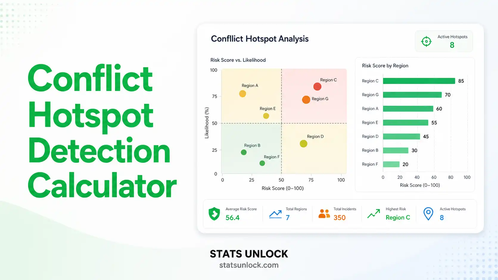
Conflict Hotspot Detection Calculator
Identify statistically significant human-wildlife conflict hotspots using Getis-Ord Gi*, Moran's I spatial autocorrelation, and kernel density estimation. Free, instant, publication-ready analysis for wildlife biologists, conservation planners, and natural resource managers.
① Data Input
Enter comma-separated or one-per-line counts of conflict incidents per spatial unit.
Supports .csv, .txt, .xlsx, .xls — headers detected automatically. Map your columns below.
Use the "Column Entry" mode in the Paste tab for a manual table-style entry. Click below to switch:
② Analysis Configuration
③ Results Summary
Getis-Ord Gi* Hotspot Statistic
The local Getis-Ord Gi* z-score for each spatial unit i is computed as:
- Gi*: Local Getis-Ord z-score for spatial unit i (hotspot statistic)
- xj: Attribute value (incident count) at unit j
- wij: Spatial weight between units i and j (1 for neighbors, 0 otherwise)
- x̄: Mean of incident counts across all units
- S: Standard deviation of incident counts
- n: Total number of spatial units in the study
- ∑: Sum across all neighboring units j
📋 Detailed Statistics
📊 Hotspot Visualizations
📈 Conflict Intensity by Spatial Unit
🔥 Getis-Ord Gi* Z-Score Distribution
🗺️ Hotspot vs Coldspot Classification
📉 Kernel Density of Conflict Counts
④ Detailed Interpretation Results
⑤ How to Write Your Results in Research
Five ready-to-use reporting templates auto-filled with your data. Click 📋 Copy on any card to grab the text.
⑥ Research Poster Panel
Conference-ready poster content auto-generated from your analysis. Copy the full text or use individual sections.
⑦ Detailed Conclusion
📐 Technical Notes — Formula Derivation & Assumptions
Extended Formula Derivation
The Getis-Ord Gi* statistic, introduced by Getis and Ord (1992) and refined by Ord and Getis (1995), is a local indicator of spatial association (LISA). It evaluates whether the sum of an attribute value within a defined neighborhood is significantly different from the sum expected under spatial randomness.
Equivalent forms:
- Numerator: Observed local sum minus expected local sum
- Denominator: Standard error of the local sum under the null hypothesis of complete spatial randomness
- Output: A standardized z-score directly comparable across spatial units
Moran's I (global autocorrelation):
I = (n / ∑∑wij) × [ ∑∑wij(xi−x̄)(xj−x̄) / ∑(xi−x̄)² ]
Assumptions
- Spatial units are properly delineated and exhaustive (no gaps, no overlaps)
- Sampling effort is approximately equal across units (or normalized as a rate)
- Conflict reporting is comparable across units (no bias in detection/reporting)
- Spatial weights (queen, rook, or distance-based) correctly reflect ecological adjacency
- Sufficient sample size (n ≥ 30 spatial units) for asymptotic normality of Gi*
Limitations
- Modifiable Areal Unit Problem (MAUP): Results can change with different grid sizes or aggregation schemes
- Edge effects: Units near the study area boundary have fewer neighbors, potentially biasing local statistics
- Reporting bias: Areas with higher human density or active monitoring may show artificial hotspots
- Temporal aggregation: Pooling multiple years can mask seasonal or annual hotspot shifts
- Causation: Hotspots indicate where conflict clusters, not why — covariate analyses are needed for mechanism
🎯 When to Use This Tool
Decision Checklist
- ✓ You have geographically referenced wildlife conflict incident counts (livestock losses, vehicle collisions, crop damage, attacks)
- ✓ You want to identify statistically significant clusters, not just visual concentrations
- ✓ You need to prioritize mitigation resources (fencing, deterrents, ranger patrols, compensation payouts)
- ✓ Your study has at least 30 spatial units with conflict count data
- ✓ You want publication-ready output for ecology, wildlife management, or conservation journals
- ✗ Do NOT use if you have only point coordinates without spatial unit aggregation (use KDE separately)
- ✗ Do NOT use if sampling/reporting effort varies drastically across units (standardize first)
- ✗ Do NOT use if your n < 30 spatial units (consider exact permutation tests instead)
Real-World Examples (USA)
- Wolf-Livestock Depredation — Rocky Mountain West: Identifying hotspots of confirmed wolf depredation on cattle and sheep across Montana, Idaho, and Wyoming to target proactive non-lethal deterrents.
- Black Bear-Human Conflict — Great Smoky Mountains: Mapping bear-incident clusters in gateway communities to focus bear-resistant trash infrastructure and visitor education.
- Mountain Lion Encounters — California Wildland-Urban Interface: Pinpointing puma encounter hotspots in Los Angeles and Bay Area suburbs for collared monitoring and outreach.
- Deer-Vehicle Collisions — Pennsylvania DOT corridors: Identifying collision hotspots along state highways to prioritize wildlife crossing structures, signage, and seasonal speed limits.
- Coyote-Pet Conflict — Chicago Metro: Detecting urban coyote conflict clusters to guide neighborhood-level hazing training and pet-owner advisories.
- Alligator-Human Encounters — Florida: Mapping nuisance alligator complaints across Lake Okeechobee watershed for trapper deployment.
Sampling Design Guidance
- Minimum 30 spatial units for reliable Gi* z-scores; ≥ 100 units preferred for Moran's I
- Grid cells of 1–5 km² typically balance resolution and sample adequacy for terrestrial mammals
- Use at least 3–5 years of pooled data unless investigating temporal hotspot shifts
- Normalize by area, road length, or human density if these confound raw counts
- Apply FDR correction (Benjamini-Hochberg) when testing many local Gi* statistics
Related Metrics — Decision Tree
Need to detect hotspots?         → Getis-Ord Gi* (this tool)
Need to detect spatial outliers? → Local Moran's I (LISA)
Need a smooth density surface?   → Kernel Density Estimation
Need to test global clustering?  → Global Moran's I or Geary's C
Have point data only?            → Ripley's K-function or nearest neighbor
Need risk/probability surface?   → MaxEnt, GLM, or Bayesian hierarchical model
📖 How to Use This Tool — Step-by-Step
- Enter Your Data: Choose Paste/Type (default), Upload CSV/Excel, or Column Entry mode. Example: 52, 48, 55, 61, 47, 8, 12, 15, ...
- Choose a Sample Dataset: Pick one of five USA-based wildlife conflict datasets to test the tool.
- Configure Analysis: Enter Study Area (e.g., "Yellowstone NP"), Species (e.g., "Gray Wolf"), Conflict Type (e.g., "Livestock Depredation"), and significance threshold (default α = 0.05).
- Click Run Hotspot Analysis: The tool computes Getis-Ord Gi* z-scores, Moran's I, and classifies each unit as Hotspot, Coldspot, or Not Significant.
- Read the Summary Cards: Green = hotspots detected (priority mitigation sites); Amber = mixed pattern; Red = no significant clustering.
- Examine the Results Table: See total incidents, mean, SD, Moran's I, z-score range, and hotspot/coldspot counts.
- Review All Four Charts: Conflict intensity, z-score distribution, classification breakdown, and density curve — each tells part of the story.
- Read the Detailed Interpretation: 5 paragraphs explaining what the values mean for your site, in plain English.
- Copy a Reporting Example: Pick the format that matches your audience — journal, thesis, policy brief, abstract, or LTER monitoring report.
- Export: Download a .txt report or full PDF for submission, sharing, or printing.
⑧ Frequently Asked Questions
What is a human-wildlife conflict hotspot?
How is the Getis-Ord Gi* statistic calculated?
What does Moran's I tell us about conflict patterns?
What sample size is needed for hotspot detection?
How do I interpret z-scores in hotspot analysis?
Can I use this tool for any wildlife species?
What is kernel density estimation in this context?
How does this differ from simple count mapping?
Should I use Getis-Ord Gi* or Local Moran's I?
How can hotspot maps inform wildlife management?
⑨ References
The following peer-reviewed and authoritative references support the statistical methods used in this calculator, covering spatial autocorrelation, wildlife conflict analysis, and best practices in conservation planning.
- Getis, A., & Ord, J. K. (1992). The analysis of spatial association by use of distance statistics. Geographical Analysis, 24(3), 189–206. https://doi.org/10.1111/j.1538-4632.1992.tb00261.x
- Ord, J. K., & Getis, A. (1995). Local spatial autocorrelation statistics: Distributional issues and an application. Geographical Analysis, 27(4), 286–306. https://doi.org/10.1111/j.1538-4632.1995.tb00912.x
- Anselin, L. (1995). Local indicators of spatial association — LISA. Geographical Analysis, 27(2), 93–115. https://doi.org/10.1111/j.1538-4632.1995.tb00338.x
- Moran, P. A. P. (1950). Notes on continuous stochastic phenomena. Biometrika, 37(1/2), 17–23. https://doi.org/10.2307/2332142
- Treves, A., & Karanth, K. U. (2003). Human-carnivore conflict and perspectives on carnivore management worldwide. Conservation Biology, 17(6), 1491–1499. https://doi.org/10.1111/j.1523-1739.2003.00059.x
- Miller, J. R. B. (2015). Mapping attack hotspots to mitigate human-carnivore conflict: Approaches and applications of spatial predation risk modeling. Biodiversity and Conservation, 24, 2887–2911. https://doi.org/10.1007/s10531-015-0993-6
- Bivand, R. S., Pebesma, E., & Gómez-Rubio, V. (2013). Applied spatial data analysis with R (2nd ed.). Springer. https://doi.org/10.1007/978-1-4614-7618-4
- Treves, A., Wallace, R. B., Naughton-Treves, L., & Morales, A. (2006). Co-managing human–wildlife conflicts: A review. Human Dimensions of Wildlife, 11(6), 383–396. https://doi.org/10.1080/10871200600984265
- Inman, R. M., Magoun, A. J., Persson, J., & Mattisson, J. (2012). The wolverine's niche: linking reproductive chronology, caching, competition, and climate. Journal of Mammalogy, 93(3), 634–644. https://doi.org/10.1644/11-MAMM-A-319.1
- Bivand, R., & Wong, D. W. S. (2018). Comparing implementations of global and local indicators of spatial association. TEST, 27(3), 716–748. https://doi.org/10.1007/s11749-018-0599-x
- U.S. Fish & Wildlife Service. (2023). Living with wildlife: National human-wildlife conflict resources. https://www.fws.gov/program/living-wildlife
- Wilson, K. R., & Anderson, D. R. (1985). Evaluation of two density estimators of small mammal population size. Journal of Mammalogy, 66(1), 13–21. https://doi.org/10.2307/1380951
- ESRI. (2024). How hot spot analysis (Getis-Ord Gi*) works. ArcGIS Pro Documentation. https://pro.arcgis.com/en/pro-app/latest/tool-reference/spatial-statistics/h-how-hot-spot-analysis-getis-ord-gi-spatial-stati.htm
- Boyce, M. S., Pitt, J., Northrup, J. M., Morehouse, A. T., Knopff, K. H., Cristescu, B., & Stenhouse, G. B. (2010). Temporal autocorrelation functions for movement rates from global positioning system radiotelemetry data. Philosophical Transactions of the Royal Society B, 365(1550), 2213–2219. https://doi.org/10.1098/rstb.2010.0080
- R Core Team. (2024). R: A language and environment for statistical computing. R Foundation for Statistical Computing. https://www.R-project.org/