Simple Linear Regression Calculator
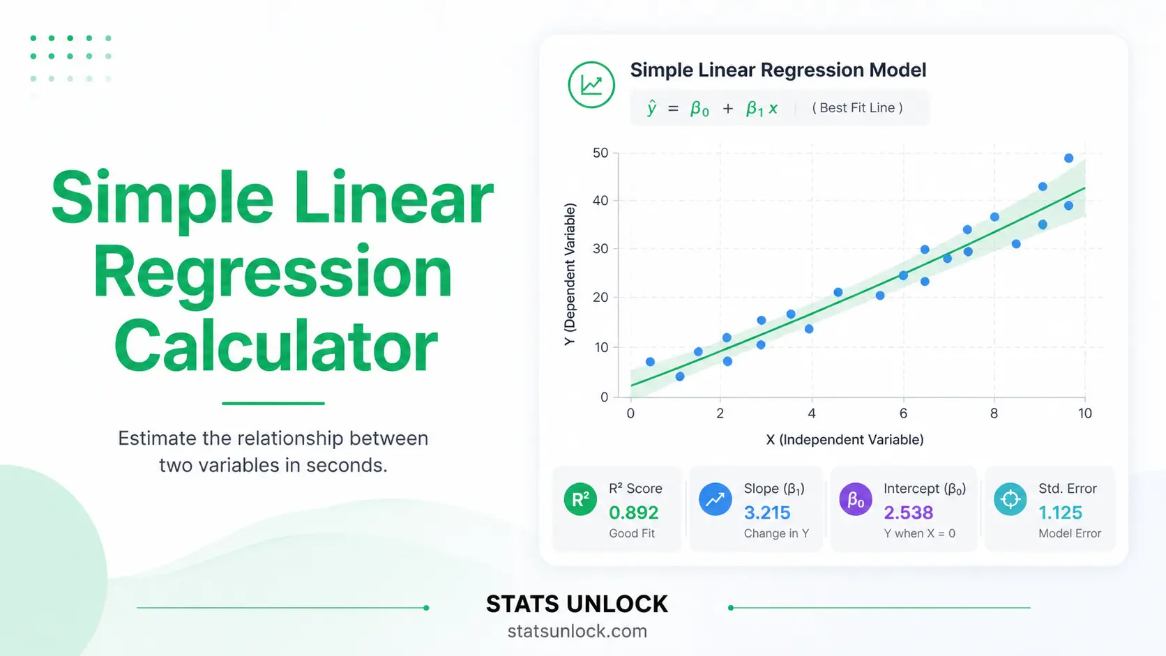
A free online linear regression calculator with graph. Paste your comma separated data, click Run, and get the least squares regression line, slope, intercept, R squared, the t test statistic, the p value, confidence intervals, assumption checks and four colour plots.
lm() and Python scipy.stats.linregress
•
Last updated:
⚡ 0. Quick Answer
A simple linear regression calculator fits the straight line Y = b0 + b1X through paired data by least squares, then reports the slope, the intercept, R squared, the t test statistic and the p value.
The slope tells you how much Y changes for a one unit rise in X. R squared tells you what share of the variation in Y the line explains. The p value tells you whether the slope is far enough from zero to be taken seriously. It does not tell you that X causes Y.
Rule of thumb: with 12 study hour and exam score pairs the line is Ŷ = 42.36 + 3.43X, R squared = 0.89, t(10) = 9.12, p < 0.001. A p value below 0.05 and a 95 percent slope interval that excludes zero mean the relationship is statistically significant.
Key takeaways
- This simple linear regression calculator returns the full least squares output: slope, intercept, R squared, standard errors, t, p and 95 percent confidence intervals.
- The slope b₁ = 3.43 in the built in example means each extra study hour predicts about 3.43 more exam points.
- R squared = 0.89 means the line explains 89 percent of the variation in exam score, and 11 percent is left to everything else.
- The test statistic is t = b₁ ÷ SE(b₁) with n − 2 degrees of freedom, and t squared equals the ANOVA F exactly.
- Always read the four diagnostic plots before trusting the p value: a curved residual plot or a funnel shape breaks the model.
📚 1. What Is Simple Linear Regression?
1.1 Plain English definition
Simple linear regression models the linear relationship between one continuous predictor (X) and one continuous outcome (Y). It estimates a slope and an intercept by ordinary least squares, which means it picks the one line that makes the sum of the squared vertical gaps between the points and the line as small as possible.
It is called simple because there is exactly one predictor. Add a second predictor and it becomes multiple linear regression. It is called linear because the model is a straight line in the parameters, not because your scatter must look perfectly straight.
1.2 What it actually measures
Three things at once. First, the direction and size of the relationship, carried by the slope. Second, the tightness of the relationship, carried by R squared and the residual standard error. Third, the evidence that the relationship is not just sampling noise, carried by the t test statistic and the p value.
1.3 A worked one liner
Twelve students recorded weekly study hours and their exam score. The mean of X is 7.50 hours and the mean of Y is 68.08 points. Sxy = 490.50 and Sxx = 143.00, so the slope is 490.50 ÷ 143.00 = 3.4301 and the intercept is 68.0833 − 3.4301 × 7.5 = 42.3578. The regression line is Ŷ = 42.36 + 3.43X.
1.4 Who uses it, and for what
Students use it in first statistics courses. Educational researchers use it to link study time to attainment. Biologists use it for dose and response, and for length and weight relationships. Economists use it for income and spending. Engineers use it for calibration curves. Health researchers use it to link a single exposure to a single continuous outcome before moving to a multivariable model.
1.5 Simple linear regression vs correlation vs multiple regression
| Method | Question it answers | Output | Choose it when |
|---|---|---|---|
| Simple linear regression | How much does Y change per unit of X? | Slope with units, intercept, R squared, prediction equation | You want to predict Y, and X is clearly the predictor |
| Pearson correlation | How strongly are X and Y linearly associated? | r from −1 to +1, unitless | Neither variable is an obvious predictor |
| Spearman correlation | Do X and Y move together in rank order? | rho, unitless | The relationship is monotonic but not straight, or there are outliers |
| Multiple linear regression | What does X add once other variables are held constant? | Partial slopes for every predictor | You have two or more predictors |
| Polynomial regression | Is the relationship curved? | Slopes for X, X squared and beyond | The residual plot shows a clear curve |
In simple linear regression, R squared is exactly the square of the Pearson correlation, so r = 0.9448 gives R squared = 0.8926.
🧮 2. Set Up Your Data
Twelve students. Weekly study hours predicting exam score.
Used in the report templates and the exported files. Leave blank for "the study site".
Values may be separated by commas, spaces, tabs or new lines. Commas are the default. X and Y must contain the same number of values.
| # | X (predictor) | Y (outcome) | Remove |
|---|
0 complete rows.
2.1 Analysis options
📊 3. Results
Enter or upload your data above, then click Run Analysis to fit the least squares regression line.
🧠 4. Interpretation of Results, In Detail
Run the analysis above and the numbers in this section fill in automatically with your own results.
4.1 What does the slope mean in simple linear regression?
The slope is the engine of the whole model. It answers one question in one number: if X goes up by one unit, how much does Y move on average? Run the analysis above to see this written out with your own values.
Three details decide whether a slope is worth reporting. The size matters in the units of your outcome, so a slope of 0.02 can be huge for a proportion and trivial for a test score. The sign tells you the direction, and a negative slope is not a weaker result, only an opposite one. The precision comes from the standard error, and a slope of 3.4 with a standard error of 3.0 is barely an estimate at all.
Never read the slope past the range of X you actually measured. If your students studied between 2 and 13 hours, the model has nothing honest to say about 40 hours. That mistake is called extrapolation and it is the single most common misuse of a regression line.
4.2 What does the intercept mean, and when is it meaningful?
The intercept is the predicted Y when X equals zero. Run the analysis to see your own intercept and whether X equal to zero is inside your data range.
An intercept is only a real prediction when X equal to zero is plausible and observed. Predicting the exam score of a student who studies zero hours is defensible if some students really did study zero hours. Predicting the weight of a person of height zero is nonsense. When zero is far outside the data, say plainly in your write up that the intercept is a mathematical anchor rather than a meaningful value. Centring X on its mean fixes this: the intercept then becomes the predicted Y at the average X, which is always interpretable.
4.3 What is a good R squared value in simple linear regression?
R squared is the share of the variation in Y that the line explains. Run the analysis to see yours.
R squared is a proportion between 0 and 1. It is computed as SSR divided by SST, which is the explained sum of squares over the total sum of squares. Multiply by 100 and you have a percentage. The leftover percentage is what the line misses, which includes every variable you did not measure plus pure measurement error.
Four things R squared does not mean. It is not the probability that the model is correct. It is not a measure of whether the model is unbiased, since a badly curved relationship can still produce a high R squared. It does not tell you that X causes Y. And it cannot be compared across datasets with different ranges of X, because widening the range of X inflates R squared without changing the underlying relationship at all.
The residual standard error is often the more useful companion number, because it carries the units of Y. Saying "our predictions are typically off by 4.5 exam points" lands better with a reader than "R squared is 0.89".
4.4 How do you calculate the simple linear regression test statistic t?
The t test statistic is the slope divided by its standard error, tested against the t distribution with n minus 2 degrees of freedom. Run the analysis to see your value.
The null hypothesis is that the true slope is exactly zero, meaning X carries no linear information about Y. A large absolute t means your estimated slope is many standard errors away from zero, which is hard to explain by sampling noise alone. The p value converts that t into a probability: the chance of seeing a slope at least this far from zero if the true slope really were zero.
A p value below your alpha means reject the null. It does not mean the effect is large, important, or causal. It also does not mean the probability that the null is true, which is the single most repeated misreading of a p value in the literature.
In simple linear regression the slope t test, the ANOVA F test and the test of the Pearson correlation are all the same test. You will find t squared equals F, exactly, every time. If they disagree in your output, something has gone wrong with the degrees of freedom.
4.5 How do you read a regression confidence interval?
The confidence interval gives the range of slope values compatible with your data. Run the analysis to see yours.
Read the interval before the p value. If the interval is [2.59, 4.27], every value inside is a defensible estimate of the true slope, and zero is nowhere near it. If the interval is [0.02, 6.40], the p value may still be under 0.05 but the honest conclusion is that you know the direction and almost nothing about the size. A narrow interval far from zero is the strong result. A wide interval that just misses zero is a call for more data, not a failed study.
4.6 How your result compares with published values
| Field | Typical R squared for one predictor | What counts as a strong result |
|---|---|---|
| Physics and engineering calibration | 0.95 to 0.999 | Anything below 0.98 usually signals an instrument problem |
| Chemistry and analytical assays | 0.98 to 0.999 | Regulatory guidance often demands R squared above 0.99 |
| Biology and physiology | 0.40 to 0.85 | Above 0.70 is a strong single predictor relationship |
| Education and psychology | 0.05 to 0.35 | Above 0.25 for one predictor is a notable finding |
| Economics and social science | 0.05 to 0.40 | Small R squared with a precise slope is still publishable |
| Ecology and field data | 0.15 to 0.60 | Field noise makes anything above 0.50 impressive |
Source bands are the conventional ranges reported in the methodological literature listed in Section 22. Compare yourself with your own field, never with 1.00.
4.7 How many data points do you need for simple linear regression?
Sample size does not change the expected slope, but it changes everything about your confidence in it. The standard error of the slope shrinks roughly with the square root of n, so quadrupling your sample halves your interval width. With n = 10 a moderate relationship often fails to reach significance. With n = 200 an almost meaningless relationship will pass easily, which is why a large study should always report the effect size and the interval rather than leaning on the p value.
The spread of X matters just as much as n. Sxx sits in the denominator of the slope standard error, so measuring across a wide range of X buys precision as effectively as adding cases. If you can choose your X values, spread them out.
4.8 What is the difference between correlation and simple linear regression?
| Comparison | What changes | Practical consequence |
|---|---|---|
| Against Pearson correlation | Regression adds units and a direction of prediction | R squared equals r squared, and the p values are identical |
| Against Spearman correlation | Spearman uses ranks, so it survives outliers and curvature | Use Spearman when the residual plot curves and you only need association |
| Against multiple regression | Other predictors are held constant | A significant simple slope can vanish once a confounder is added |
| Against polynomial regression | Curvature is modelled explicitly | Use it when the residual plot shows a clear U or arch shape |
| Against robust regression | Outliers are down weighted rather than squared | Use it when one or two points dominate Cook's distance |
4.9 The decision guide
- Look at the scatter plot first. If it is not roughly a straight cloud, stop and rethink the model.
- Check the residual plot for curvature and for a funnel shape.
- Check the Q-Q plot for heavy tails, which weaken the p value in small samples.
- Only now read the p value for the slope.
- Read the confidence interval and decide whether the size is practically important.
- Report R squared and the residual standard error together, never R squared alone.
- State plainly that the design, not the regression, decides whether you may talk about causes.
4.10 Common mistakes this calculator prevents
| Mistake | Why it happens | What this tool does |
|---|---|---|
| Swapping X and Y | Regression is not symmetric, unlike correlation | The input fields are labelled predictor and outcome, and the equation shows which is which |
| Using n minus 1 degrees of freedom | Copied from the one sample t test | Degrees of freedom are fixed at n minus 2 and shown in the output |
| Reporting R squared with no error term | R squared looks impressive on its own | The residual standard error is shown beside it as a summary card |
| Ignoring a curved residual plot | The p value looked fine | The linearity check fails loudly and the residual plot is shown by default |
| Extrapolating far past the data | The equation happily accepts any number | Predictions outside the observed X range are flagged as extrapolation |
| Treating p equal to 0.06 as "no effect" | Alpha is treated as a wall | Borderline results get an amber badge, not a red one |
| Dropping an inconvenient outlier | It improves R squared | Influential points are flagged so you have to justify the decision in writing |
✍ 5. How to Write Your Results in Research
Every template below fills in with your own numbers once you click Run Analysis. Click Copy on the one that matches where you are writing. Before the run they show underscores.
5.1 What a complete regression report contains
A reader who never sees your data should be able to reconstruct your conclusion from the sentence alone. That needs six ingredients: the model test (F with both degrees of freedom), the model fit (R squared), the coefficient (b with its standard error), the coefficient test (t with its degrees of freedom), the exact p value, and the confidence interval. Leave any one of them out and a reviewer will ask for it.
5.2 How do you report simple linear regression in APA format?
APA conventions for regression
- Italicise the statistical symbols: F, t, p, R2, b, SE.
- Drop the leading zero on anything that cannot exceed one, so write .89 and .001, not 0.89 and 0.001.
- Report exact p values to two or three decimals, and write p < .001 only when it really is smaller.
- Give both degrees of freedom for F, as F(1, 10), and one for t, as t(10).
- Report the unstandardised b for a single predictor. The standardised beta equals r here, so it adds nothing.
5.3 Thesis or dissertation
Thesis conventions
- Name the software and version in the Methods chapter, and say which assumption checks you ran.
- State the alpha level once, in Methods, and do not repeat it for every test.
- Put the scatter plot with the fitted line in the Results chapter, and the diagnostic plots in an appendix.
- Write the regression equation on its own line with the standard errors underneath in brackets.
5.4 Plain language for a non technical reader
Plain language conventions
- Lead with the practical size, not the p value.
- Translate the slope into a familiar step, for example per extra hour or per extra 10 units.
- Say "linked to" or "predicted", never "caused", unless you ran an experiment.
- Give the typical prediction error in real units instead of quoting R squared.
5.5 Structured abstract or conference poster
Abstract conventions
- One sentence each for design, sample, main result and conclusion.
- Numbers go inside the sentence, not into a separate table.
- Always include n, the coefficient, the interval and the p value.
- On a poster, put the equation and R squared directly on the scatter plot.
5.6 Replication or pre-registration
Pre-registration conventions
- Fix alpha, the tail direction and the exclusion rules before you look at the data.
- Name the exact model, the transformation if any, and the software.
- State the smallest effect size of interest, not just the null.
- Say in advance what you will do if an assumption fails, for example switch to Spearman.
5.7 Table and figure conventions
| Element | What to show | Common reviewer complaint |
|---|---|---|
| Coefficient table | b, SE, t, df, p, and the confidence interval, one row per term | Confidence interval missing |
| Model line | R squared, adjusted R squared, residual standard error, F and its two df | Only R squared given |
| Scatter figure | Raw points, fitted line, axis labels with units, n in the caption | Axes unlabelled or units missing |
| Diagnostics | Residuals vs fitted and a Q-Q plot, usually in an appendix | Assumptions claimed but never shown |
| Decimals | Two or three for coefficients, three for p, two for R squared | Six decimals copied straight from software |
5.8 Final reporting checklist
- Sample size n, and how many cases were dropped and why.
- The regression equation with both coefficients.
- Standard error for the slope.
- t, its degrees of freedom, and the exact p value.
- The confidence interval for the slope with its confidence level.
- R squared and the residual standard error.
- F with both degrees of freedom for the model test.
- A sentence naming which assumptions you checked and how.
- A sentence limiting the conclusion to the observed range of X.
- A statement that association is not causation, unless the design earns it.
∑ 6. Formulas Used
Seven formulas do all the work in simple linear regression. They are shown in the order a reader needs them: the line first, then the pieces it is built from, then the tests and intervals around it.
📝 7. How to Use This Simple Linear Regression Calculator
- Name the group. Type a name in the cluster name box, for example
Class A. The name is editable at any time and appears in every chart, table and report template. - Enter the predictor X. Paste your X values as comma separated numbers, for example
2, 3, 4, 5, 6, 7. Spaces, tabs and new lines also work. - Enter the outcome Y. Paste the matching Y values in the same order. The two lists must have the same count or the tool will tell you.
- Or upload a file. Open the Upload tab, pick a CSV or Excel file, click one numeric column as X, then click the columns that should each become a cluster.
- Add more clusters. Click Add cluster to compare several regressions side by side, for example one per school or per field site.
- Set your options. Choose alpha, the tail direction and the number of decimal places. Two tailed is the default and is what most journals expect.
- Optionally set a prediction X. Type a value in the prediction box to get Ŷ with its confidence and prediction intervals.
- Click Run Analysis. Nothing is calculated before you click. The results, the interpretation, the report templates and the conclusion all fill in at once.
- Check the assumptions. Read the four plots and the assumption panel. A red badge means the p value cannot be trusted as it stands.
- Export. Click Download Doc for a plain text report you can paste into a manuscript, or Download PDF for a printable copy.
Worked example. Load sample dataset 1, leave alpha at 0.05, and click Run. You should see Ŷ = 42.3578 + 3.4301X, R squared = 0.8926, t(10) = 9.1158 and p < 0.001. If you see anything different, one of the two value lists has an extra or a missing number.
📈 8. How to Calculate Simple Linear Regression in Excel
Excel handles simple linear regression better than most people expect. Four built in functions give you the whole line in seconds, and the Analysis ToolPak gives you the full table with t statistics and p values. What trips people up is that the direct functions take the ranges in the order Y first, then X, which is the opposite of how you read the equation.
=SLOPE(B2:B13,A2:A13) and =INTERCEPT(B2:B13,A2:A13). Those two numbers are your regression line.8.1 The functions you need
| You want | Excel function | Note |
|---|---|---|
| Slope b₁ | =SLOPE(known_ys, known_xs) | Y range first. This is the most common mistake in the whole section. |
| Intercept b₀ | =INTERCEPT(known_ys, known_xs) | Same argument order as SLOPE. |
| R squared | =RSQ(known_ys, known_xs) | Equals =CORREL()^2 exactly in simple regression. |
| Correlation r | =CORREL(array1, array2) | Symmetric, so argument order does not matter here. |
| Residual standard error s | =STEYX(known_ys, known_xs) | Uses n minus 2 in the denominator, exactly as this calculator does. |
| Sample size n | =COUNT(A2:A13) | COUNT skips text and blanks, which silently changes n. |
| Sxx | =DEVSQ(A2:A13) | The sum of squared deviations of X from its mean. |
| Sxy | =SUMPRODUCT(A2:A13-AVERAGE(A2:A13),B2:B13-AVERAGE(B2:B13)) | Confirm the slope by hand: Sxy divided by Sxx. |
| Standard error of the slope | =STEYX(B2:B13,A2:A13)/SQRT(DEVSQ(A2:A13)) | No single built in function exists for this. |
| t statistic for the slope | =SLOPE(...)/SE_cell | Build it in two steps so you can see both parts. |
| p value, two tailed | =T.DIST.2T(ABS(t_cell), n-2) | T.DIST.2T requires a positive first argument, so wrap it in ABS. |
| Critical t at 95 percent | =T.INV.2T(0.05, n-2) | 2.2281 for 10 degrees of freedom. |
| Predicted Y at a new X | =FORECAST.LINEAR(new_x, known_ys, known_xs) | Identical to =TREND() for one predictor. |
| Everything at once | =LINEST(known_ys, known_xs, TRUE, TRUE) | Returns a 5 by 2 array with coefficients, standard errors, R squared, s, F and df. |
| Full table with p values | Data → Data Analysis → Regression | Analysis ToolPak. It must be enabled first under File, Options, Add-ins. |
8.2 Step by step
1 Lay the data out in two columns
Put the predictor X in column A and the outcome Y in column B, with one header row. Every row is one case, so row 2 is student 1.
A1: Study hours (X) B1: Exam score (Y)The first eight of twelve rows. Study hours run 2 to 13 and scores run 52 to 90. Keep both columns numeric, with no units typed into the cells.
2 Get the slope, the intercept and R squared
In a free area of the sheet, type the four direct functions. Remember that the Y range comes first inside each one.
=SLOPE(B2:B13,A2:A13) · =INTERCEPT(B2:B13,A2:A13) =RSQ(B2:B13,A2:A13) · =STEYX(B2:B13,A2:A13)The slope is 3.4301, the intercept is 42.3578, R squared is 0.8926 and the residual standard error is 4.4996. The regression line is Y = 42.36 + 3.43X.
3 Build the standard error, the t statistic and the p value
Excel has no single function for the standard error of a slope, so assemble it from STEYX and DEVSQ. Then divide the slope by it and convert to a p value.
SE(b₁) = =STEYX(B2:B13,A2:A13)/SQRT(DEVSQ(A2:A13)) t = =F2/F6 · p = =T.DIST.2T(ABS(F7),10)Sxx is 143.0000, so SE(b₁) is 4.4996 ÷ √143 = 0.3763. That gives t = 3.4301 ÷ 0.3763 = 9.1158 on 10 degrees of freedom, and a two tailed p of 0.0000037.
4 Or use the Analysis ToolPak for the whole table at once
Go to Data, then Data Analysis, then Regression. Set the Y Range to B1:B13 and the X Range to A1:A13, tick Labels, tick Residuals and Normal Probability Plots, then choose an output range.
Data → Data Analysis → Regression → Y Range B1:B13, X Range A1:A13, Labels ✓The ToolPak returns Multiple R = 0.9448, R Square = 0.8926, Adjusted R Square = 0.8818, Standard Error = 4.4996 and n = 12, with the coefficient block giving the same slope of 3.4301, SE 0.3763 and t 9.1158 that you built by hand in step 3.
5 Add fitted values and residuals so you can plot the diagnostics
Anchor the two coefficient cells with dollar signs, then fill both columns down. The residual column is what you plot against the fitted column.
C2: =$F$3+$F$2*A2 · D2: =B2-C2 then fill down to row 13Row 2 fits 49.2180 against an observed 54, leaving a residual of +4.7820. The residuals must sum to zero across all twelve rows, which is a fast way to catch a typing error.
8.3 The awkward cases in Excel
| Awkward case | What to type | The classic mistake |
|---|---|---|
| Standard error of the intercept | =STEYX(B2:B13,A2:A13)*SQRT(1/COUNT(A2:A13)+AVERAGE(A2:A13)^2/DEVSQ(A2:A13)) | People reuse the slope standard error, which is a different number entirely. |
| One tailed p value | =T.DIST.RT(t_cell, n-2) | Halving the two tailed p is only correct when the sign of t matches your hypothesis. |
| Confidence interval for the slope | =b1 ± T.INV.2T(0.05,10)*SE_cell | Using 1.96 instead of the t critical value, which is too narrow at small n. |
| Reading LINEST output | Select a 5 by 2 range, type =LINEST(B2:B13,A2:A13,TRUE,TRUE), press Ctrl+Shift+Enter in older Excel | The slope sits top left and the intercept top right, which is the reverse of the reading order. |
| Degrees of freedom | =COUNT(A2:A13)-2 | Typing n minus 1, copied from the one sample t test. |
| Prediction interval | Build it from s, n, Sxx and the distance of the new X from the mean | Using the confidence interval for the mean response, which is far too narrow for a single new case. |
8.4 Why your Excel answer might differ from R or Python
| Situation | What happens | Fix |
|---|---|---|
| Blank cells inside a range | COUNT quietly shrinks n while SLOPE pairs the remaining values, so the two disagree | Delete incomplete rows entirely rather than clearing single cells |
| Numbers stored as text | They are skipped, so your n falls without warning | Use =ISNUMBER(A2) down the column, or Text to Columns to convert |
| Missing values coded as 0 or 999 | Excel treats them as real data and drags the slope | Replace them with truly empty cells first, then delete the rows |
| Rounding shown versus rounding stored | Excel displays 3.43 but stores 3.4300699... | Compare full precision values, never the displayed ones |
| Ranges of unequal length | SLOPE returns #N/A | X and Y must have the same count, which this calculator enforces |
| ToolPak p value shown as 3.69E-06 | Scientific notation is easy to misread as 3.69 | Report it as p < .001 in APA style |
With clean data, Excel, R, Python and this calculator all agree to at least four decimal places for simple linear regression. Unlike the t-test, there is no competing default here, because there is only one ordinary least squares fit.
8.5 Charting the result in Excel
Select both data columns, then Insert, Scatter, and pick the plain markers option with no connecting lines. Right click any point, choose Add Trendline, pick Linear, and tick both Display Equation on chart and Display R-squared value on chart. Two formatting changes make it publication ready: delete the automatic chart title and the gridlines, and label both axes with their units. For the residual plot, chart column D against column C using the same scatter type, then add a horizontal line at zero.
8.6 Excel errors you will probably hit
| Error | Cause | Fix |
|---|---|---|
#DIV/0! | Every X value is the same, so Sxx is zero | The predictor must vary. Check for a filled down constant. |
#N/A | The X and Y ranges have different lengths | Make both ranges cover exactly the same rows. |
#VALUE! | Text inside a numeric range, often a stray unit like "hrs" | Strip units out of the cells and keep them in the header only. |
#NUM! | T.DIST.2T was given a negative t | Wrap the t reference in ABS(). |
#REF! | A row referenced by the formula was deleted | Rebuild the formula against the current range. |
| Data Analysis missing | The Analysis ToolPak is not enabled | File, Options, Add-ins, Manage Excel Add-ins, Go, tick Analysis ToolPak. |
📈 9. How to Calculate Simple Linear Regression in R
In R the whole model is one line, lm(y ~ x), but the one liner is rarely what you should report. The script below fits the model, prints every number a journal will ask for, checks all five assumptions, and saves one publication ready figure at 300 dpi.
Rscript regression.R. The only line you need to change is the one that defines x and y at the top.No installation is needed. Base R alone does everything here, which is exactly what reviewers expect to see in a methods section.
9.1 The complete script
simple_linear_regression.R
# Simple linear regression calculator, base R only
# Fits Y = b0 + b1*X by ordinary least squares and checks every assumption

set.seed(42)  # reproducible jitter in the figure

# ---- 1. YOUR DATA. Change only these two lines ------------------------
x <- c(2, 3, 4, 5, 6, 7, 8, 9, 10, 11, 12, 13)   # predictor: study hours
y <- c(54, 52, 53, 52, 63, 71, 70, 75, 79, 76, 90, 82)  # outcome: exam score

# From a CSV instead:
# dat <- read.csv("mydata.csv")
# dat <- dat[complete.cases(dat$hours, dat$score), ]   # drop rows with NA
# x <- dat$hours ; y <- dat$score

xlab <- "Study hours per week"
ylab <- "Exam score"
alpha <- 0.05

# ---- 2. CLEAN AND CHECK ----------------------------------------------
ok <- complete.cases(x, y)
x  <- x[ok]; y <- y[ok]
n  <- length(x)
if (n < 3)      stop("Need at least 3 complete pairs.")
if (var(x) == 0) stop("The predictor does not vary, so no slope exists.")

# ---- 3. FIT THE MODEL -------------------------------------------------
fit  <- lm(y ~ x)
s    <- summary(fit)
ci   <- confint(fit, level = 1 - alpha)
av   <- anova(fit)

b0   <- coef(fit)[1]
b1   <- coef(fit)[2]
se1  <- s$coefficients[2, 2]
tval <- s$coefficients[2, 3]
pval <- s$coefficients[2, 4]
r2   <- s$r.squared
adj  <- s$adj.r.squared
rse  <- s$sigma
fst  <- s$fstatistic[1]
df2  <- n - 2
res  <- resid(fit)
fitv <- fitted(fit)

# ---- 4. ASSUMPTION CHECKS --------------------------------------------
sw   <- shapiro.test(res)                       # normality of residuals
dw   <- sum(diff(res)^2) / sum(res^2)        # Durbin-Watson, want near 2
bp   <- summary(lm(res^2 ~ fitv))$r.squared * n  # Breusch-Pagan LM statistic
bp_p <- pchisq(bp, df = 1, lower.tail = FALSE)
cook <- cooks.distance(fit)
infl <- which(cook > 4 / n)

# ---- 5. PRINTED REPORT -----------------------------------------------
cat("\n================ SIMPLE LINEAR REGRESSION ================\n")
cat(sprintf("n                    : %d\n", n))
cat(sprintf("Equation             : Y = %.4f + %.4f * X\n", b0, b1))
cat(sprintf("Slope b1 (SE)        : %.4f (%.4f)\n", b1, se1))
cat(sprintf("t(%d)                 : %.4f\n", df2, tval))
cat(sprintf("p value              : %.6f\n", pval))
cat(sprintf("%.0f%% CI for slope    : [%.4f, %.4f]\n", 100*(1-alpha), ci[2,1], ci[2,2]))
cat(sprintf("R squared / adjusted : %.4f / %.4f\n", r2, adj))
cat(sprintf("Residual std error   : %.4f on %d df\n", rse, df2))
cat(sprintf("F(1, %d)              : %.4f\n", df2, fst))
cat("---------------- assumption checks ----------------------\n")
cat(sprintf("Shapiro-Wilk p       : %.4f  (want above 0.05)\n", sw$p.value))
cat(sprintf("Durbin-Watson        : %.4f  (want 1.5 to 2.5)\n", dw))
cat(sprintf("Breusch-Pagan p      : %.4f  (want above 0.05)\n", bp_p))
cat(sprintf("Influential points   : %s\n",
    if (length(infl)) paste(infl, collapse = ", ") else "none"))

# ---- 6. PLAIN ENGLISH VERDICT ----------------------------------------
verdict <- if (pval < alpha) {
  sprintf("p is %.5f, below %.2f, so the slope differs significantly from zero. Each extra unit of X predicts a change of %.4f in Y, and the model explains %.1f%% of the variation.",
          pval, alpha, b1, 100 * r2)
} else {
  sprintf("p is %.5f, not below %.2f, so there is not enough evidence that the slope differs from zero.", pval, alpha)
}
cat("\nVERDICT: ", verdict, "\n\n", sep = "")

# ---- 7. ONE 300 dpi FIGURE, FOUR PANELS ------------------------------
png("simple_linear_regression.png", width = 2400, height = 2000, res = 300)
par(mfrow = c(2, 2), mar = c(4.2, 4.2, 2.6, 1))

plot(x, y, pch = 19, col = "#2563eb", xlab = xlab, ylab = ylab,
     main = "1. Scatter with least squares line")
abline(fit, col = "#16a34a", lwd = 3)
legend("topleft", bty = "n", cex = 0.9,
       legend = sprintf("Y = %.2f + %.2f X\nR2 = %.3f", b0, b1, r2))

plot(fitv, res, pch = 19, col = "#9333ea", xlab = "Fitted values",
     ylab = "Residuals", main = "2. Residuals vs fitted")
abline(h = 0, lty = 2, col = "#c2410c", lwd = 2)
lines(lowess(fitv, res), col = "#0d9488", lwd = 2)

qqnorm(res, pch = 19, col = "#0d9488", main = "3. Normal Q-Q of residuals")
qqline(res, col = "#c2410c", lwd = 2)

hist(res, breaks = "FD", col = "#bbf7d0", border = "#15803d",
     xlab = "Residual", main = "4. Histogram of residuals")
abline(v = 0, lty = 2, col = "#c2410c", lwd = 2)

dev.off()
cat("Figure saved as simple_linear_regression.png (300 dpi)\n")
cat("Generated by STATS UNLOCK - statsunlock.com\n")
9.2 What each part does
| Line or function | What it does and why it is there |
|---|---|
| complete.cases(x, y) | Drops any pair where either value is NA. Without it, lm silently drops rows and your reported n is wrong. |
| var(x) == 0 | Stops with a clear message when the predictor is constant, instead of returning a mysterious NA slope. |
| lm(y ~ x) | Fits the ordinary least squares model. The tilde reads as "y modelled by x". |
| summary(fit) | Holds the coefficient matrix, R squared, adjusted R squared, sigma and the F statistic. |
| s$coefficients[2, ] | Row 2 is the slope. Row 1 is the intercept. Columns are estimate, standard error, t and p. |
| confint(fit) | Uses the t distribution with n minus 2 df, not the normal, which matters at small n. |
| anova(fit) | Gives SSR, SSE and the F test. Confirm that F equals t squared. |
| shapiro.test(res) | Tests normality of the residuals, not of Y. Testing Y itself is a common error. |
| sum(diff(res)^2)/sum(res^2) | Durbin-Watson by hand, so no extra package is needed. Values near 2 mean no autocorrelation. |
| cooks.distance(fit) | Flags points whose removal would move the line. The 4/n rule is the usual screening threshold. |
| lowess(fitv, res) | Adds a smoother to the residual plot so curvature is visible rather than imagined. |
| png(..., res = 300) | Saves at journal resolution. Without res = 300 the text in the figure comes out tiny. |
9.3 What the figure shows
Panel 1 is the result: the points and the fitted line with the equation and R squared printed in the corner. Panel 2 is the honesty check, and the teal smoother should stay flat along zero. If it arches, the relationship is curved and a straight line is the wrong model. Panel 3 puts the residuals against a normal reference line, and a slight wobble at the ends is normal in small samples while a strong S shape is not. Panel 4 should look roughly symmetric and centred on zero.
9.4 Common R problems and fixes
| Problem | Cause | Fix |
|---|---|---|
| Coefficient shows as NA | The predictor is constant or perfectly collinear | Check var(x) before fitting |
| n in the output is smaller than expected | lm dropped rows with NA silently | Filter with complete.cases first and print length(x) |
| Error: object 'x' not found | The data live in a data frame that was never attached | Use lm(score ~ hours, data = dat) instead of bare vectors |
| shapiro.test errors out | Fewer than 3 or more than 5000 residuals | Use a Q-Q plot for very small or very large samples |
| The p value differs from SPSS | A different number of cases survived listwise deletion | Compare n first, then the coefficients |
| The figure file is empty | dev.off() was never called | Always pair png() with dev.off() |
| Slope looks inverted | x and y were swapped in the formula | The outcome always goes on the left of the tilde |
| summary prints stars but no p | The p value is below 2e-16 | Report p < .001 and read the exact value from s$coefficients[2,4] |
9.5 Useful one-liners
coef(lm(y ~ x))                                  # just the intercept and slope
confint(lm(y ~ x), level = 0.99)                   # 99 percent interval
predict(lm(y ~ x), data.frame(x = 7.5), interval = "prediction")
predict(lm(y ~ x), data.frame(x = 7.5), interval = "confidence")
cor.test(x, y)                                     # same p value as the slope test
summary(lm(y ~ I(x - mean(x))))                    # centred, so the intercept is meaningful
write.csv(data.frame(x, y, fit = fitted(fit), res = resid(fit)), "regression_output.csv")
plot(fit)                                          # the four standard base R diagnostics
📈 10. How to Calculate Simple Linear Regression in Python
Python gives you two honest routes. scipy.stats.linregress returns the slope, intercept, r, p and standard error in a single call, which is perfect for a quick check. For anything you plan to publish, use statsmodels, which prints the full coefficient table, the ANOVA and the confidence intervals in the layout a journal expects.
regression.py and run python regression.py, or paste it into a Jupyter cell. Change only the two data lines at the top.Install once with pip install numpy scipy matplotlib pandas. Nothing else is required.
10.1 The complete script
regression.py
# Simple linear regression calculator in Python
# Fits Y = b0 + b1*X by ordinary least squares and checks every assumption

import numpy as np
import matplotlib.pyplot as plt
from scipy import stats

np.random.seed(42)  # reproducible figure

# ---- 1. YOUR DATA. Change only these two lines ------------------------
x = np.array([2, 3, 4, 5, 6, 7, 8, 9, 10, 11, 12, 13], dtype=float)
y = np.array([54, 52, 53, 52, 63, 71, 70, 75, 79, 76, 90, 82], dtype=float)

# From a CSV instead:
# import pandas as pd
# dat = pd.read_csv("mydata.csv").dropna(subset=["hours", "score"])
# x = dat["hours"].to_numpy(float); y = dat["score"].to_numpy(float)

xlab, ylab = "Study hours per week", "Exam score"
alpha = 0.05

# ---- 2. CLEAN AND CHECK ----------------------------------------------
mask = ~(np.isnan(x) | np.isnan(y))
x, y = x[mask], y[mask]
n = x.size
if n < 3:
    raise ValueError("Need at least 3 complete pairs.")
if np.var(x) == 0:
    raise ValueError("The predictor does not vary, so no slope exists.")

# ---- 3. FIT THE MODEL -------------------------------------------------
res = stats.linregress(x, y)
b1, b0 = res.slope, res.intercept
fitted = b0 + b1 * x
resid = y - fitted

df2 = n - 2
sxx = np.sum((x - x.mean()) ** 2)
sse = np.sum(resid ** 2)
sst = np.sum((y - y.mean()) ** 2)
ssr = sst - sse
mse = sse / df2
rse = np.sqrt(mse)                       # residual standard error
se1 = rse / np.sqrt(sxx)                 # standard error of the slope
se0 = rse * np.sqrt(1 / n + x.mean() ** 2 / sxx)
tval = b1 / se1
pval = 2 * stats.t.sf(abs(tval), df2)
tcrit = stats.t.ppf(1 - alpha / 2, df2)
ci = (b1 - tcrit * se1, b1 + tcrit * se1)
r2 = ssr / sst
adj = 1 - (1 - r2) * (n - 1) / df2
fstat = ssr / mse
pf = stats.f.sf(fstat, 1, df2)

# ---- 4. ASSUMPTION CHECKS --------------------------------------------
sw_p = stats.shapiro(resid).pvalue if 3 <= n <= 5000 else float("nan")
dw = np.sum(np.diff(resid) ** 2) / sse
bp_r2 = stats.linregress(fitted, resid ** 2).rvalue ** 2
bp_p = stats.chi2.sf(n * bp_r2, 1)
lev = 1 / n + (x - x.mean()) ** 2 / sxx
cook = (resid ** 2 / (2 * mse)) * (lev / (1 - lev) ** 2)
infl = np.where(cook > 4 / n)[0] + 1

# ---- 5. PRINTED REPORT -----------------------------------------------
print("\n================ SIMPLE LINEAR REGRESSION ================")
print(f"n                    : {n}")
print(f"Equation             : Y = {b0:.4f} + {b1:.4f} * X")
print(f"Slope b1 (SE)        : {b1:.4f} ({se1:.4f})")
print(f"Intercept b0 (SE)    : {b0:.4f} ({se0:.4f})")
print(f"t({df2})                 : {tval:.4f}")
print(f"p value              : {pval:.6f}")
print(f"{100*(1-alpha):.0f}% CI for slope    : [{ci[0]:.4f}, {ci[1]:.4f}]")
print(f"R squared / adjusted : {r2:.4f} / {adj:.4f}")
print(f"Residual std error   : {rse:.4f} on {df2} df")
print(f"F(1, {df2})              : {fstat:.4f}  (p = {pf:.6f})")
print("---------------- assumption checks ----------------------")
print(f"Shapiro-Wilk p       : {sw_p:.4f}  (want above 0.05)")
print(f"Durbin-Watson        : {dw:.4f}  (want 1.5 to 2.5)")
print(f"Breusch-Pagan p      : {bp_p:.4f}  (want above 0.05)")
print(f"Influential rows     : {list(infl) if infl.size else 'none'}")

# ---- 6. PLAIN ENGLISH VERDICT ----------------------------------------
if pval < alpha:
    verdict = (f"p is {pval:.5f}, below {alpha:.2f}, so the slope differs significantly "
               f"from zero. Each extra unit of X predicts a change of {b1:.4f} in Y, "
               f"and the model explains {100*r2:.1f}% of the variation.")
else:
    verdict = (f"p is {pval:.5f}, not below {alpha:.2f}, so there is not enough "
               f"evidence that the slope differs from zero.")
print("\nVERDICT:", verdict, "\n")

# ---- 7. ONE 300 dpi FIGURE, FOUR PANELS ------------------------------
fig, ax = plt.subplots(2, 2, figsize=(11, 9))

ax[0, 0].scatter(x, y, color="#2563eb", s=45, zorder=3)
xs = np.linspace(x.min(), x.max(), 100)
ax[0, 0].plot(xs, b0 + b1 * xs, color="#16a34a", lw=3)
ax[0, 0].set(xlabel=xlab, ylabel=ylab, title="1. Scatter with least squares line")
ax[0, 0].text(0.04, 0.92, f"Y = {b0:.2f} + {b1:.2f}X\nR2 = {r2:.3f}",
              transform=ax[0, 0].transAxes, va="top", fontsize=10)

ax[0, 1].scatter(fitted, resid, color="#9333ea", s=45)
ax[0, 1].axhline(0, ls="--", color="#c2410c", lw=2)
ax[0, 1].set(xlabel="Fitted values", ylabel="Residuals", title="2. Residuals vs fitted")

stats.probplot(resid, dist="norm", plot=ax[1, 0])
ax[1, 0].set_title("3. Normal Q-Q of residuals")

ax[1, 1].hist(resid, bins="auto", color="#bbf7d0", edgecolor="#15803d")
ax[1, 1].axvline(0, ls="--", color="#c2410c", lw=2)
ax[1, 1].set(xlabel="Residual", ylabel="Frequency", title="4. Histogram of residuals")

fig.tight_layout()
fig.savefig("simple_linear_regression.png", dpi=300, bbox_inches="tight")
print("Figure saved as simple_linear_regression.png (300 dpi)")
print("Generated by STATS UNLOCK - statsunlock.com")
10.2 What each part does
| Line or function | What it does and why it is there |
|---|---|
| dtype=float | Forces floating point. Integer arrays cause silent truncation in older NumPy code. |
| ~(np.isnan(x) | np.isnan(y)) | Drops any pair with a missing value. np.mean returns nan if even one value is nan, so this must come first. |
| stats.linregress(x, y) | Returns slope, intercept, rvalue, pvalue and stderr in one call. Its p value is always two tailed. |
| rse = sqrt(sse / (n - 2)) | The residual standard error. Note the n minus 2, which matches Excel's STEYX and R's sigma. |
| se1 = rse / sqrt(sxx) | The slope standard error, built by hand so you can see where it comes from. |
| 2 * stats.t.sf(abs(t), df) | The two tailed p value. sf is the survival function, which is more accurate in the far tail than 1 minus cdf. |
| stats.t.ppf(1 - alpha/2, df) | The critical t value. Using 1.96 instead is the classic small sample error. |
| np.var(x) | Defaults to ddof=0, the population variance. For a sample standard deviation matching R and Excel, pass ddof=1. |
| stats.shapiro(resid) | Tests the residuals, never the raw Y values. |
| lev and cook | Leverage and Cook's distance computed directly, so statsmodels is not needed. |
| stats.probplot | Draws the Q-Q plot straight onto a matplotlib axis. |
| dpi=300, bbox_inches="tight" | Journal resolution with no clipped axis labels. |
10.3 What the figure shows
The four panels answer four questions in order. Is there a relationship, and how steep is it? Is a straight line the right shape? Are the residuals close enough to normal for the p value to mean what it claims? And is the spread of errors symmetric, or is one long tail doing all the work? Read them in that order, and only trust the p value once panels 2, 3 and 4 look reasonable.
10.4 Common Python problems and fixes
| Problem | Cause | Fix |
|---|---|---|
| Everything comes out nan | A single nan in the arrays poisons np.mean and np.sum | Apply the mask shown in step 2, or use np.nanmean |
| Standard deviation differs from Excel | np.std defaults to ddof=0 | Use np.std(x, ddof=1) for the sample value |
| ValueError: shapes not aligned | x and y have different lengths | Print x.size and y.size before fitting |
| p value prints as 0.0 | The true value is below machine precision | Report p < .001 and print with scientific notation if you need the exact value |
| statsmodels gives a different R squared | The constant was never added | Wrap with sm.add_constant(x) before fitting OLS |
| The figure is blank in a script | plt.show() was called before savefig | Always save before showing |
| Plots look pixelated in a document | The default dpi is 100 | Pass dpi=300 to savefig |
| Slope has the wrong sign | linregress was called as linregress(y, x) | The predictor always comes first in linregress |
10.5 Useful one-liners
from scipy import stats
stats.linregress(x, y)                          # slope, intercept, r, p, stderr
np.polyfit(x, y, 1)                             # [slope, intercept], no inference
stats.pearsonr(x, y)                            # same p value as the slope test
stats.spearmanr(x, y)                           # rank based fallback when linearity fails

import statsmodels.api as sm
m = sm.OLS(y, sm.add_constant(x)).fit(); print(m.summary())
print(m.conf_int(alpha=0.05))                    # confidence intervals
print(m.get_prediction([1, 7.5]).summary_frame())  # prediction at X = 7.5
Running it. Save the script and run python regression.py from a terminal. In Jupyter, drop the savefig line and add plt.show() instead. Both routes give identical numbers.
📋 11. Reference Tables
11.1 Critical t values for the slope test, df = n − 2
| n | df = n − 2 | t at α = 0.10 (two tailed) | t at α = 0.05 (two tailed) | t at α = 0.01 (two tailed) |
|---|---|---|---|---|
| 5 | 3 | 2.353 | 3.182 | 5.841 |
| 6 | 4 | 2.132 | 2.776 | 4.604 |
| 7 | 5 | 2.015 | 2.571 | 4.032 |
| 10 | 8 | 1.860 | 2.306 | 3.355 |
| 12 | 10 | 1.812 | 2.228 | 3.169 |
| 17 | 15 | 1.753 | 2.131 | 2.947 |
| 20 | 18 | 1.734 | 2.101 | 2.878 |
| 30 | 28 | 1.701 | 2.048 | 2.763 |
| 50 | 48 | 1.677 | 2.011 | 2.682 |
| 100 | 98 | 1.661 | 1.984 | 2.627 |
| 202 | 200 | 1.653 | 1.972 | 2.601 |
| 502 | 500 | 1.648 | 1.965 | 2.586 |
What to conclude: if your absolute t exceeds the tabled value at your alpha, reject the null of zero slope. With n = 12 the 0.05 threshold is 2.228, and the worked example t of 9.116 is far beyond it. Note how slowly the critical value falls after n = 30, which is why the jump from n = 10 to n = 30 buys you far more than the jump from n = 100 to n = 500.
11.2 Critical F values for the model test, df = 1 and n − 2
| df2 = n − 2 | F at α = 0.05 | F at α = 0.01 | √F at α = 0.05, which equals the critical t |
|---|---|---|---|
| 3 | 10.13 | 34.12 | 3.182 |
| 5 | 6.61 | 16.26 | 2.571 |
| 10 | 4.96 | 10.04 | 2.228 |
| 15 | 4.54 | 8.68 | 2.131 |
| 20 | 4.35 | 8.10 | 2.086 |
| 30 | 4.17 | 7.56 | 2.042 |
| 50 | 4.03 | 7.17 | 2.009 |
| 100 | 3.94 | 6.90 | 1.984 |
| 200 | 3.89 | 6.76 | 1.972 |
What to conclude: the last column proves the identity that catches people out. In simple linear regression the F test and the slope t test are the same test, and F is exactly t squared. If your software reports an F whose square root is not your t, one of the two used the wrong degrees of freedom.
11.3 Interpreting R squared by field
| R squared | Variance explained | General label | Typical home |
|---|---|---|---|
| 0.00 to 0.05 | 0 to 5 percent | Negligible | Almost any noisy field |
| 0.05 to 0.15 | 5 to 15 percent | Small but often meaningful | Social science, epidemiology |
| 0.15 to 0.35 | 15 to 35 percent | Moderate | Psychology, education |
| 0.35 to 0.65 | 35 to 65 percent | Substantial | Ecology, physiology |
| 0.65 to 0.90 | 65 to 90 percent | Strong | Biology, controlled experiments |
| 0.90 to 1.00 | 90 to 100 percent | Very strong, or suspicious | Physics, calibration curves |
What to conclude: R squared above 0.98 in behavioural data usually means the two variables are two measurements of the same thing, not a discovery. Judge against your own field, and always report the residual standard error beside it. Bands follow the conventions summarised by Cohen (1988) and the field surveys listed in Section 22.
11.4 Critical correlation r for significance at α = 0.05, two tailed
| n | Critical r | Equivalent minimum R squared | Reading |
|---|---|---|---|
| 5 | 0.878 | 0.771 | Only enormous relationships can reach significance |
| 10 | 0.632 | 0.399 | Still very demanding |
| 15 | 0.514 | 0.264 | Moderate relationships start to be detectable |
| 20 | 0.444 | 0.197 | A practical working minimum for teaching datasets |
| 30 | 0.361 | 0.130 | Comfortable for a moderate effect |
| 50 | 0.279 | 0.078 | Small effects become detectable |
| 100 | 0.197 | 0.039 | Very small effects reach significance |
| 200 | 0.139 | 0.019 | Statistical significance stops implying importance |
What to conclude: the same relationship is significant at n = 100 and not significant at n = 10. That is why a non significant result in a small study is weak evidence of absence, and why a significant result in a huge study needs an effect size before it means anything.
11.5 Sample size needed for 80 percent power at α = 0.05
| True correlation r | True R squared | Effect label | n needed |
|---|---|---|---|
| 0.10 | 0.01 | Very small | 781 |
| 0.20 | 0.04 | Small | 193 |
| 0.30 | 0.09 | Small to moderate | 84 |
| 0.40 | 0.16 | Moderate | 46 |
| 0.50 | 0.25 | Moderate to large | 28 |
| 0.60 | 0.36 | Large | 18 |
| 0.70 | 0.49 | Very large | 13 |
| 0.80 | 0.64 | Extremely large | 9 |
What to conclude: plan your sample from the smallest effect you would care about, not from the effect you hope to see. If a correlation of 0.20 would still matter in your field, you need roughly 193 cases, and a study of 30 will almost certainly miss it.
11.6 Assumption check thresholds used by this calculator
| Check | Statistic | Pass | Caution | Fail |
|---|---|---|---|---|
| Normality of residuals | Normality test p (D'Agostino-Pearson in this tool, Shapiro-Wilk in R and Python) | above 0.05 | 0.01 to 0.05 | below 0.01 |
| Constant variance | Breusch-Pagan p | above 0.05 | 0.01 to 0.05 | below 0.01 |
| Independence | Durbin-Watson | 1.5 to 2.5 | 1.0 to 1.5 or 2.5 to 3.0 | below 1.0 or above 3.0 |
| Linearity | Correlation of residuals with X squared | |r| below 0.30 | 0.30 to 0.50 | above 0.50 |
| Influence | Cook's distance | all below 4 ÷ n | one point above 4 ÷ n | any point above 1.0 |
| Sample size | n | 30 or more | 10 to 29 | below 10 |
What to conclude: a caution badge does not invalidate your result, it tells you to mention the issue in the limitations. A fail badge means the p value as printed cannot be defended, and you should either transform the data, switch to a robust or rank based method, or explain very clearly why you proceeded anyway.
11.7 Durbin-Watson quick guide
| DW value | Meaning | What to do |
|---|---|---|
| 0.0 to 1.0 | Strong positive autocorrelation | Errors run in streaks. Use a time series model instead. |
| 1.0 to 1.5 | Mild positive autocorrelation | Report it and check whether the data were collected in order. |
| 1.5 to 2.5 | No meaningful autocorrelation | The independence assumption is satisfied. |
| 2.5 to 3.0 | Mild negative autocorrelation | Often an artefact of small n. Note it and continue. |
| 3.0 to 4.0 | Strong negative autocorrelation | Residuals alternate in sign. Check for a periodic pattern or an over corrected series. |
What to conclude: the Durbin-Watson statistic only makes sense when your rows have a meaningful order, such as time or spatial sequence. For a shuffled cross sectional sample it carries no information, and you should judge independence from the study design instead.
📈 12. Example Results (8 Worked Cases)
Eight real shaped datasets, each fitted with the same least squares method this calculator uses. They deliberately span the full range of outcomes, from a textbook fit to a model that should not be reported at all. Every figure is drawn from the actual numbers in the table beside it.
Study hours and exam score
The built in sample dataset, and the numbers used in Sections 8, 9 and 10.
Twelve students recorded their weekly study hours and sat the same exam. The question is how much a single extra hour of study is worth in exam points.
| Quantity | Value |
|---|---|
| Slope b₁ (SE) | 3.4301 (0.3763) |
| Intercept b₀ | 42.3578 |
| t(10) | 9.1158 |
| p value | 0.0000037 |
| R squared / residual SE | 0.8926 / 4.4996 |
| 95 percent CI for slope | [2.5917, 4.2685] |
What it means: each additional study hour predicts about 3.43 more exam points, and study hours explain 89 percent of the differences in score. Typical prediction error is 4.5 points.
How to write it: A simple linear regression significantly predicted exam score from weekly study hours, F(1, 10) = 83.10, p < .001, R² = .89, b = 3.43, SE = 0.38, t(10) = 9.12, 95% CI [2.59, 4.27].
Nitrogen dose and grain yield
A designed agronomy trial with three replicates at each of six doses.
Eighteen field plots received nitrogen at 0, 20, 40, 60, 80 or 100 kilograms per hectare. Yield was measured at harvest in tonnes per hectare.
| Quantity | Value |
|---|---|
| Slope b₁ (SE) | 0.0426 (0.0032) |
| t(16) | 13.1621 |
| p value | < 0.001 |
| R squared / residual SE | 0.9155 / 0.4694 |
| 95 percent CI for slope | [0.0358, 0.0495] |
What it means: each extra kilogram of nitrogen per hectare adds about 0.043 tonnes per hectare, so 100 kilograms adds roughly 4.3 tonnes. Because the doses were assigned by the experimenter, this result does support a causal claim.
How to write it: Nitrogen dose significantly predicted grain yield, b = 0.043 t/ha per kg/ha, SE = 0.003, t(16) = 13.16, p < .001, R² = .92, 95% CI [0.036, 0.049].
Evening screen time and sleep duration
A p value just under alpha, which is exactly where careful reporting matters most.
Twenty adults logged evening screen time and average nightly sleep for one week. The slope is negative, but only barely significant.
| Quantity | Value |
|---|---|
| Slope b₁ (SE) | −0.0438 (0.0198) |
| t(18) | −2.2109 |
| p value | 0.0402 |
| R squared / residual SE | 0.2136 / 0.5114 |
| 95 percent CI for slope | [−0.0855, −0.0022] |
What it means: the interval nearly touches zero, so the honest reading is that the direction is probably negative and the size is very poorly estimated. Ten extra hours of weekly screen time is associated with somewhere between 0.02 and 0.86 fewer hours of sleep, which is almost the whole plausible range.
How to write it: Evening screen time was a significant but weak predictor of sleep duration, b = −0.044, SE = 0.020, t(18) = −2.21, p = .040, R² = .21, 95% CI [−0.086, −0.002]. The interval is wide and a replication with a larger sample is needed.
Shoe size and IQ score
What a genuine absence of relationship looks like on the page.
Twenty four adults were measured for shoe size and completed a standard IQ test. There is no reason to expect a relationship, and none is found.
| Quantity | Value |
|---|---|
| Slope b₁ (SE) | −0.0157 (0.8813) |
| t(22) | −0.0179 |
| p value | 0.9859 |
| R squared / residual SE | 0.0000 / 12.2684 |
| 95 percent CI for slope | [−1.8434, 1.8119] |
What it means: there is no detectable linear relationship. Note that the interval is wide and symmetric around zero, so this is a study that failed to detect anything rather than a study that proved nothing exists.
How to write it: Shoe size did not significantly predict IQ score, b = −0.02, SE = 0.88, t(22) = −0.02, p = .986, R² < .001, 95% CI [−1.84, 1.81]. The wide interval means small effects cannot be ruled out at this sample size.
Calibration curve for a spectrophotometer
Only six points, but an almost perfect fit, which is normal for instruments.
Six standards of known concentration were read at 595 nanometres to build a calibration curve for later unknown samples.
| Quantity | Value |
|---|---|
| Slope b₁ (SE) | 0.0578 (0.0005) |
| t(4) | 121.1445 |
| p value | < 0.001 |
| R squared / residual SE | 0.9997 / 0.0040 |
| 95 percent CI for slope | [0.0564, 0.0591] |
What it means: absorbance rises by 0.0578 units per milligram per litre. With R squared of 0.9997 the curve is fit for purpose. Anything below 0.99 in this setting points to a pipetting or instrument problem, not to an interesting biological finding.
How to write it: The calibration curve was linear across 0 to 10 mg/L, absorbance = 0.008 + 0.0578 × concentration, R² = .9997, residual SE = 0.004, t(4) = 121.14, p < .001.
Daily activity and a heart rate proxy in 300 adults
A tiny p value hiding a modest effect. This is the large sample trap.
Three hundred adults wore a step counter for a month. The p value is minuscule, but the model explains only about an eighth of the variation.
| Quantity | Value |
|---|---|
| Slope b₁ (SE) | 0.5866 (0.0896) |
| t(298) | 6.5456 |
| p value | < 0.001 |
| R squared / residual SE | 0.1257 / 14.2042 |
| 95 percent CI for slope | [0.4102, 0.7630] |
What it means: the relationship is real, but 87 percent of the variation is unexplained and the residual standard error of 14.2 is larger than the whole predicted range across the middle of the data. Report the effect size prominently, or a reader will assume p below .001 means a strong relationship.
How to write it: Activity significantly predicted the heart rate proxy, b = 0.59, SE = 0.09, t(298) = 6.55, p < .001, but explained only 12.6 percent of the variance, R² = .13, 95% CI [0.41, 0.76].
Household income and annual spending
A textbook funnel. The slope is fine, the standard error is not.
Forty households reported income and total annual spending. Spending varies far more among high earners than among low earners, which is a classic case of non constant variance.
| Quantity | Value |
|---|---|
| Slope b₁ (SE) | 0.8463 (0.1552) |
| t(38) | 5.4539 |
| p value | < 0.001 |
| R squared / residual SE | 0.4391 / 14.5249 |
| Shapiro-Wilk p on residuals | 0.0010 |
What it means: the slope estimate is still unbiased, but the standard error, the confidence interval and the p value are all untrustworthy. Fix it by taking logs of both variables, by using weighted least squares, or by reporting heteroscedasticity robust standard errors.
How to write it: Income predicted spending, b = 0.85, t(38) = 5.45, p < .001, R² = .44. Residual variance increased with fitted value, so a log-log model was fitted and is reported as the primary analysis.
Body length and body mass in a fish population
A strong biological relationship measured in the field.
Twenty six fish were measured for standard length and weighed. Length and mass relationships like this are used to estimate biomass from length alone.
| Quantity | Value |
|---|---|
| Slope b₁ (SE) | 5.5795 (0.2063) |
| t(24) | 27.0407 |
| p value | < 0.001 |
| R squared / residual SE | 0.9682 / 2.2878 |
| 95 percent CI for slope | [5.1536, 6.0053] |
What it means: each extra centimetre of length predicts about 5.58 grams of mass across the 11.5 to 19.0 centimetre range sampled. The negative intercept is not a real prediction, because a fish of zero length does not exist, and it simply anchors the line inside the measured range.
How to write it: Standard length significantly predicted body mass, b = 5.58 g/cm, SE = 0.21, t(24) = 27.04, p < .001, R² = .97, 95% CI [5.15, 6.01]. Predictions are valid only within the sampled length range of 11.5 to 19.0 cm.
🧪 13. Data Collection Protocol
Design statement. Simple linear regression assumes one continuous predictor and one continuous outcome measured on the same independent units. Each row is one unit. The predictor may be observed, as in a survey, or set by the researcher, as in a dose response experiment. Only the second design supports a causal claim.
13.1 How to collect data for a simple linear regression calculator
- Define the unit of analysis. One student, one plot, one patient, one site. Write it down before collecting anything, because it decides what independence means.
- Define the predictor X precisely. Name the variable, its units and its measurement instrument. "Study hours" is not enough. "Self reported hours of solo study per week, excluding class time" is.
- Define the outcome Y the same way. Same level of detail, same care about units.
- Decide the range of X you need. Spread matters as much as sample size, because Sxx sits in the denominator of the slope standard error. Deliberately sample low, middle and high X values.
- Choose the sample size before collecting. Use Table 11.5 and the smallest effect you would care about. Write the number into your protocol.
- Randomise where you can. If you control X, assign the levels at random across units. If you only observe X, randomise which units you sample.
- Measure X and Y independently. The person measuring Y should not know the X value, wherever that is practical, to prevent expectancy effects.
- Record every case, including the awkward ones. Do not drop a unit because it looks unusual. Record it and decide later, in writing.
- Log the order of collection. This is what lets you interpret the Durbin-Watson statistic honestly.
- Record missing values as blank, never as 0 or 999. A numeric missing code silently drags the slope.
- Keep the raw file untouched. Do all cleaning in a copy, with a script or a documented list of changes.
- Check the data entry. Re-enter a random 10 percent and compare. Transposed digits are the single most common source of an influential outlier.
13.2 How to structure your data for regression analysis
The calculator expects exactly two numeric lists of equal length. In a spreadsheet that means two columns and one header row.
| Student ID | Study hours (X) | Exam score (Y) | Collection order |
|---|---|---|---|
| S01 | 2 | 54 | 1 |
| S02 | 3 | 52 | 2 |
| S03 | 4 | 53 | 3 |
The ID column is for your own audit trail and is ignored by the calculator. Do not type units into the value cells, and never merge cells.
13.3 Minimum sample size for a simple linear regression study
Three pairs is the mathematical minimum, because you need at least one residual degree of freedom. It is not a usable minimum. For a moderate relationship, around r = 0.4, you need roughly 46 cases for 80 percent power at alpha 0.05. For a small relationship, around r = 0.2, you need roughly 193. Below n = 20 the confidence interval for the slope is usually so wide that the study cannot settle anything.
13.4 Pre-registration line
Copy this into your pre-registration, then fill in the blanks before you collect any data: "We will fit a simple linear regression of [outcome] on [predictor] using ordinary least squares, testing the slope against zero with a two tailed t test at alpha = 0.05 on n minus 2 degrees of freedom. Our target sample size is [n], chosen for 80 percent power to detect a slope corresponding to r = [r]. If the residual plot shows non constant variance or the Shapiro-Wilk test on residuals gives p below 0.01, we will report the log transformed model as the primary analysis and the untransformed model in a supplement."
13.5 Common mistakes that make the data unusable
| Mistake | Why it ruins the analysis |
|---|---|
| Measuring the same person more than once and treating the rows as independent | Independence fails, standard errors are too small, and the p value is meaningless. Use a mixed model. |
| Recording X only at two extreme values | You cannot detect curvature, so you cannot check linearity at all. |
| Rounding X heavily, for example to the nearest 5 hours | Attenuates the slope towards zero and inflates the residual variance. |
| Coding missing as 0 | Adds fake points at X or Y equal to zero, which have enormous leverage. |
| Mixing two units in one column, such as kilograms and pounds | Creates two invisible populations and a meaningless slope. |
| Discarding cases after seeing the scatter plot | Turns exploratory choice into a fabricated p value. |
| Using an ordinal outcome such as a 1 to 5 rating as if it were continuous | Residuals cannot be normal and are strongly patterned. Use ordinal regression. |
🎯 14. When to Use This Calculator
This free simple linear regression calculator is designed for anyone who needs one continuous predictor, one continuous outcome and a defensible published style output. Use the checklists below before you run anything.
14.1 Use it when
- You have exactly one predictor and one outcome, both measured on a continuous scale.
- Each row is a different independent unit.
- The scatter plot looks broadly like a straight band, even a noisy one.
- You want a prediction equation, not just a strength of association number.
- You need slope, intercept, R squared, t, p and confidence intervals in one place.
- You need APA or thesis ready wording you can paste straight into a manuscript.
14.2 Do not use it when
- Your outcome is binary, such as pass or fail. Use logistic regression.
- Your outcome is a count, such as number of visits. Use Poisson or negative binomial regression.
- Your outcome is an ordered rating from 1 to 5. Use ordinal regression.
- You have two or more predictors you need to control for. Use multiple linear regression.
- The same units were measured repeatedly over time. Use a mixed model or a time series model.
- The scatter is clearly curved. Use polynomial regression or transform a variable.
- Your predictor is a group label rather than a number. Use a t-test or ANOVA.
14.3 Four real world examples
| Field | Predictor X | Outcome Y | Typical question |
|---|---|---|---|
| Education | Weekly study hours | Exam score | How many points is one extra hour of study worth? |
| Agronomy | Nitrogen applied, kg/ha | Grain yield, t/ha | What is the marginal yield return per kilogram of fertiliser? |
| Clinical chemistry | Known concentration | Instrument absorbance | Is the calibration curve linear across the working range? |
| Ecology | Body length, cm | Body mass, g | Can biomass be estimated from length alone in the field? |
14.4 Study design guidance
If you can set X yourself, do so, and spread the levels evenly across the widest range that is still realistic. Replicate at each level so you can separate pure error from lack of fit. If you can only observe X, sample deliberately across its range rather than taking whatever is convenient, since a convenience sample clustered in the middle gives you a small Sxx and a wide confidence interval for no extra cost.
14.5 Decision tree: is simple linear regression the right test?
- Is the outcome continuous? If no, go to logistic, Poisson or ordinal regression.
- Is the predictor continuous? If no, and it is a group label, use a t-test for two groups or ANOVA for more.
- Is there exactly one predictor? If no, use multiple linear regression.
- Are the rows independent? If no, use a mixed model.
- Is the scatter roughly straight? If no, transform a variable or use polynomial regression.
- Do you only need strength of association, not a prediction equation? If yes, Pearson correlation is simpler and answers the question.
- Do outliers dominate the plot? If yes, consider Spearman correlation or robust regression.
- If you reached this line, simple linear regression is the right choice.
🔧 15. Troubleshooting and Common Errors
The tool says X and Y have different counts
Cause: a trailing comma, a blank line, or one value pasted twice. The most common culprit is a stray comma at the end of one list.
Fix: count the values in each box. The tool shows the count under each field once you type. Remove trailing separators and re-paste.
The slope comes out as zero or the tool refuses to run
Cause: every X value is identical, so Sxx is zero and the slope is undefined.
Fix: the predictor has to vary. Check that you did not fill a column down with a constant, and that you did not paste the same list into both boxes.
The slope has the opposite sign to what I expected
Cause: X and Y were swapped, or one list was pasted in reverse order while the other was not.
Fix: check the scatter plot. If the cloud slopes the way you expected but the number does not, the lists are misaligned. Regression is not symmetric, so order matters.
R squared is very high but the residual plot is curved
Cause: a strong curved relationship still produces a high R squared, because a straight line captures most of a gentle curve.
Fix: trust the residual plot over R squared. Add a squared term, or take logs of one or both variables, then compare the residual plots.
One point sits far away from the rest and changes everything
Cause: a high leverage point, usually an extreme X value, or a data entry error such as a transposed digit.
Fix: check the raw record first. If it is a genuine observation, report the analysis both with and without it, and say which one you treat as primary. Never delete it silently.
The p value is significant but the confidence interval is enormous
Cause: a large slope estimate with a large standard error, typical of a small sample with a wide spread.
Fix: report the interval prominently and describe the size as poorly estimated. Collect more data before drawing a practical conclusion.
My Excel answer differs from R and Python
Cause: almost always a different n. Excel silently skips text and blanks, so a column with one value stored as text quietly loses a case.
Fix: print n in all three before comparing anything else. See Section 8.4 for the full list.
The Shapiro-Wilk test fails but the Q-Q plot looks fine
Cause: with a large sample, Shapiro-Wilk detects trivially small departures from normality that do not affect the inference.
Fix: above n of about 100, judge normality from the Q-Q plot and the histogram rather than from the test. Regression is robust to mild non normality at large n.
The Durbin-Watson statistic is far from 2
Cause: the rows have a meaningful order and the errors are correlated, or the rows have no meaningful order and the statistic is noise.
Fix: if your data are a time series, move to a time series model. If they are cross sectional and shuffled, ignore the statistic and justify independence from your design.
The prediction at my chosen X looks absurd
Cause: extrapolation. The equation happily accepts any number, including values far outside the range you measured.
Fix: only predict inside the observed range of X. The tool flags a prediction as extrapolation when it falls outside that range.
The uploaded file loads but every column is greyed out
Cause: the columns are not numeric, usually because of a unit suffix, a thousands separator, or a currency symbol inside the cells.
Fix: strip everything except digits, a decimal point and a minus sign, then re-upload. Keep units in the header row only.
Nothing happens when I click Run Analysis
Cause: a validation message is waiting above the button, usually about a non numeric value or mismatched counts.
Fix: scroll up to the message area under the options and fix the item it names. The tool never computes on invalid input, and it never shows a bare NaN.
⚖ 16. Assumptions and Limitations
16.1 What are the assumptions of simple linear regression?
- Linearity. Requires the mean of Y to be a straight line function of X. Check with the scatter plot and the residuals versus fitted plot. If it fails, the slope is a biased summary of a curved relationship, and predictions at the two ends of the X range are systematically wrong in opposite directions.
- Independence of errors. Requires each observation to carry its own information. Check with the study design first, and with the Durbin-Watson statistic when the rows have a meaningful order. If it fails, standard errors are usually too small, so p values are too small and confidence intervals too narrow.
- Constant variance, also called homoscedasticity. Requires the spread of residuals to be the same across the fitted range. Check with the residuals versus fitted plot and the Breusch-Pagan test. If it fails, the slope stays unbiased but its standard error is wrong, usually too small at the high variance end, which inflates significance.
- Approximate normality of residuals. Requires residuals, not raw Y values, to be roughly normal. Check with the Q-Q plot, the histogram and the Shapiro-Wilk test. If it fails at small n, the p value and the confidence interval are unreliable. At large n the central limit theorem largely rescues the inference.
- No extreme influential points. Requires no single case to control the slope. Check with Cook's distance against the 4 divided by n rule and with leverage. If it fails, the slope reflects one observation rather than the sample, and the direction of the bias is toward that one point.
- The predictor is measured without substantial error. Requires X to be reliable. Check with the reliability of your instrument. If it fails, the slope is biased toward zero, an effect called regression dilution, so a real relationship looks weaker than it is.
16.2 Limitations
- It cannot establish causation. Use a randomised experiment, or a design with a credible identification strategy such as instrumental variables or a regression discontinuity.
- It handles only one predictor. A confounder can create or hide the whole relationship. Use multiple linear regression when other variables matter.
- It is not robust to outliers. Squaring the residuals gives extreme points enormous weight. Use robust regression, such as an M estimator, or Theil-Sen regression.
- It cannot model a curve. Use polynomial regression, a spline, or a generalised additive model.
- It assumes an additive constant effect. If the effect of X depends on a third variable, you need an interaction term, which requires multiple regression.
- Predictions are only valid inside the observed range of X. There is no statistical method that fixes extrapolation. Collect data across the range you care about.
- It treats the outcome as unbounded. With a proportion or a percentage the model can predict values below 0 or above 100. Use beta regression or a logit transformation.
- R squared can be inflated by a wide X range. Two studies of the same relationship can report very different R squared values purely because of sampling. Compare slopes across studies, not R squared.
🏁 17. Conclusion
17.1 What was found
Run the analysis above and a plain summary of your own result appears here, with the equation, the effect size and the p value written out in sentences.
17.2 What it means in practice
This block translates the slope into a practical statement about your own units once you click Run Analysis.
17.3 Cautions
The assumption checks are summarised here after the run, together with what each failure would do to the p value.
17.4 Next steps
Suggested next analyses appear here after the run, chosen from what your own diagnostics show.
17.5 The short version
A simple linear regression calculator turns two columns of numbers into a sentence you can defend. The slope gives the size and direction, the confidence interval gives the precision, R squared and the residual standard error give the fit, and the four diagnostic plots decide whether any of it can be trusted. Report all of them together, keep your predictions inside the range you measured, and be careful never to promote a significant slope into a causal claim your design cannot support. Used that way, the simple linear regression calculator is one of the most reliable tools in applied statistics.
❓ 18. Frequently Asked Questions (20)
What is a simple linear regression calculator?
A simple linear regression calculator fits a straight line through paired X and Y data using the least squares method. It returns the slope, the intercept, R squared, the standard error, the t test statistic, the p value and the confidence intervals, so you can say how strongly one variable predicts another.
How do you calculate simple linear regression?
Calculate the mean of X and the mean of Y. Then compute Sxy, the sum of the products of the deviations, and Sxx, the sum of the squared X deviations. The slope is b₁ = Sxy divided by Sxx, and the intercept is b₀ = the mean of Y minus b₁ times the mean of X. That pair of numbers is the least squares regression line.
What is the formula for the least squares regression line?
The fitted line is Ŷ = b₀ + b₁X, where b₁ = Sxy ÷ Sxx and b₀ = ȳ − b₁x̄. Least squares chooses b₀ and b₁ so that the sum of the squared vertical distances between the observed points and the line is as small as possible.
What does the slope mean in simple linear regression?
The slope is the average change in Y for a one unit increase in X. If the slope is 3.43 for study hours predicting exam score, then one extra hour of study is associated with about 3.43 more score points on average.
What does the intercept mean in simple linear regression?
The intercept is the predicted value of Y when X is zero. It is only meaningful when X equal to zero is inside or near the range of your data. If nobody in your sample had X equal to zero, treat the intercept as a mathematical anchor, not a real prediction.
What is a good R squared value in simple linear regression?
There is no universal cut off. In laboratory or physical measurement work R squared above 0.90 is common. In psychology, education and ecology, values of 0.10 to 0.40 can still be publishable. Judge R squared against the typical values in your own field, not against 1.00. Table 11.3 gives the usual bands.
How do you calculate the simple linear regression test statistic t?
Divide the slope by its standard error: t = b₁ ÷ SE(b₁). Compare that t against the t distribution with n minus 2 degrees of freedom. In simple linear regression this t squared equals the ANOVA F statistic exactly.
What p value means the regression is significant?
By convention a p value below 0.05 means the slope is significantly different from zero. A p value of 0.049 and a p value of 0.051 carry almost the same evidence, so report the exact p value and the confidence interval rather than only the significant or not significant label.
What is the difference between correlation and simple linear regression?
Correlation gives one unitless number describing the strength and direction of a linear association, and it treats X and Y symmetrically. Simple linear regression gives a predictive equation with units, treats X as the predictor and Y as the outcome, and lets you forecast Y at a new X. In simple linear regression, R squared is exactly the square of the Pearson correlation.
How many data points do you need for simple linear regression?
You need at least three points to have any residual degrees of freedom, but that is a mathematical minimum and not a useful one. Aim for at least 20 to 30 observations for a stable slope, and more if the relationship is weak or the data are noisy. Table 11.5 gives the sample sizes needed for 80 percent power.
What are the assumptions of simple linear regression?
Five assumptions matter: the relationship is linear, the observations are independent, the residuals have constant variance, the residuals are approximately normal, and there are no extreme influential points. This calculator checks all five and shows a pass, caution or fail badge for each.
What is a residual plot and what should it look like?
A residual plot shows the residuals on the vertical axis against the fitted values on the horizontal axis. A healthy plot looks like a formless cloud centred on zero with the same vertical spread all the way across. A curve means the relationship is not linear, and a funnel shape means the variance is not constant.
How do you read a regression confidence interval?
A 95 percent confidence interval for the slope gives the range of slope values that are compatible with your data. If the interval excludes zero, the slope is significant at the 0.05 level. A wide interval means the slope is poorly estimated even when the p value is small.
How to calculate simple linear regression in Excel?
Use =SLOPE(Y range, X range) and =INTERCEPT(Y range, X range) for the line, =RSQ() for R squared and =STEYX() for the standard error of the estimate. For the full output with t statistics and p values, use Data, Data Analysis, Regression from the Analysis ToolPak, which must be enabled first. Section 8 walks through it with screenshots.
How do you run simple linear regression in R?
Fit the model with fit <- lm(y ~ x) and read the output with summary(fit). Add confint(fit) for the confidence intervals and plot(fit) for the four standard diagnostic plots. R uses n minus 2 degrees of freedom for the slope test, the same as this calculator. Section 9 has a complete runnable script.
How do you run simple linear regression in Python?
The quickest route is scipy.stats.linregress(x, y), which returns the slope, intercept, r value, p value and standard error in one call. For the full table with an ANOVA and confidence intervals, use statsmodels with sm.OLS(y, sm.add_constant(x)).fit() and print the summary. Section 10 has a complete script.
Can simple linear regression prove causation?
No. Regression measures association only. A significant slope tells you that Y changes in step with X in your sample. Causation needs a design that rules out confounders and reverse causation, such as a randomised experiment or a well identified natural experiment.
What is the standard error of the estimate in regression?
The standard error of the estimate, also called the residual standard error, is the typical size of a prediction error in the units of Y. It is the square root of the sum of squared residuals divided by n minus 2. Smaller is better, and it is easier to interpret than R squared because it carries units.
How do you report simple linear regression in APA format?
Report the model test, the coefficient and the effect size together, for example: A simple linear regression significantly predicted exam score from study hours, F(1, 10) = 83.10, p < .001, R2 = .89. Each additional hour of study predicted a 3.43 point increase in score, b = 3.43, SE = 0.38, t(10) = 9.12, p < .001, 95% CI [2.59, 4.27].
Is this simple linear regression calculator free?
Yes. This simple linear regression calculator online is completely free, needs no sign up, and runs entirely in your browser. Your data never leaves your device, which makes it safe for unpublished or confidential research data.
📑 19. Cite This Tool
Stats Unlock. (2026). Simple linear regression calculator [Online statistical tool]. https://statsunlock.com/simple-linear-regression-calculator
@misc{statsunlock_slr_2026,
  title  = {Simple Linear Regression Calculator},
  author = {{Stats Unlock}},
  year   = {2026},
  note   = {Online statistical tool},
  url    = {https://statsunlock.com/simple-linear-regression-calculator/}
}
Run the analysis above to generate a Methods paragraph filled with your own values.
🔗 20. Related Tools
Add a second predictor when a confounder needs to be held constant. The natural next step from this page.
The unitless companion. Identical p value, no prediction equation, and r squared here equals R squared there.
Use it when the residual plot shows a curve and a straight line is the wrong shape.
The rank based fallback when outliers dominate the scatter or the relationship is monotonic but not straight.
The fix when the Breusch-Pagan check fails and the residuals fan out across the fitted range.
Plot X against Y before you fit anything. If the cloud is not roughly straight, stop and rethink the model.
All six links point to live StatsUnlock tools. Each one is the tool you move to when this page tells you simple linear regression is the wrong choice.
📖 21. Glossary of Terms
| Term | Plain meaning |
|---|---|
| Adjusted R squared | R squared with a small penalty for the number of parameters estimated. In simple regression it is always slightly below R squared. |
| Alpha | The cut off you choose in advance for calling a result significant, usually 0.05. |
| ANOVA table | A table splitting the total variation in Y into the part the line explains and the part left over. |
| Breusch-Pagan test | A test of whether the spread of the residuals changes across the fitted range. |
| Confidence interval | A range of values for a quantity that are compatible with the data, at a stated confidence level. |
| Cook's distance | A measure of how much the fitted line would move if one particular case were removed. |
| Degrees of freedom | The number of independent pieces of information left after estimating the parameters. Here it is n minus 2. |
| Durbin-Watson statistic | A number near 2 when consecutive residuals are unrelated, and far from 2 when they run in patterns. |
| Extrapolation | Using the equation to predict outside the range of X you actually measured. |
| Fitted value | The value the line predicts for a case, written Ŷ. |
| Heteroscedasticity | The spread of the residuals changing across the range, usually a funnel shape. |
| Homoscedasticity | The spread of the residuals staying the same across the range, which is what the model assumes. |
| Influential point | A single case whose removal noticeably changes the slope. |
| Intercept | The predicted Y when X is zero, written b₀. |
| Least squares | The rule that picks the line making the sum of squared vertical gaps as small as possible. |
| Leverage | How far a case sits from the mean of X. High leverage cases can pull the line hard. |
| Ordinary least squares (OLS) | The standard least squares method, with every case weighted equally. |
| Outcome | The variable you are trying to predict, Y. Also called the response or dependent variable. |
| p value | The probability of seeing a result at least this extreme if the true slope were zero. |
| Predictor | The variable you predict from, X. Also called the explanatory or independent variable. |
| Q-Q plot | A plot comparing your residuals against what a normal distribution would look like. |
| R squared | The proportion of the variation in Y that the line explains, from 0 to 1. |
| Residual | The gap between an observed Y and the value the line predicts for it. |
| Residual standard error | The typical size of a residual, in the units of Y. Also called the standard error of the estimate. |
| Shapiro-Wilk test | A test of whether a set of numbers, here the residuals, could have come from a normal distribution. |
| Slope | The average change in Y for a one unit rise in X, written b₁. |
| Standard error | The typical amount an estimate would vary from sample to sample. |
| Sum of squares | A total of squared distances, used to split variation into explained and unexplained parts. |
| t statistic | An estimate divided by its standard error, compared against the t distribution. |
📚 22. References
Twenty peer reviewed journal articles behind the methods, thresholds and interpretation bands used by this simple linear regression calculator. Every entry has a resolvable DOI.
- Aiken, L. S., West, S. G., & Millsap, R. E. (2008). Doctoral training in statistics, measurement, and methodology in psychology. American Psychologist, 63(1), 32-50. https://doi.org/10.1037/0003-066X.63.1.32
- Altman, D. G., & Bland, J. M. (1995). Statistics notes: The normal distribution. BMJ, 310(6975), 298. https://doi.org/10.1136/bmj.310.6975.298
- Anscombe, F. J. (1973). Graphs in statistical analysis. The American Statistician, 27(1), 17-21. https://doi.org/10.1080/00031305.1973.10478966
- Belsley, D. A. (1984). Demeaning conditioning diagnostics through centering. The American Statistician, 38(2), 73-77. https://doi.org/10.1080/00031305.1984.10483169
- Breusch, T. S., & Pagan, A. R. (1979). A simple test for heteroscedasticity and random coefficient variation. Econometrica, 47(5), 1287-1294. https://doi.org/10.2307/1911963
- Cohen, J. (1992). A power primer. Psychological Bulletin, 112(1), 155-159. https://doi.org/10.1037/0033-2909.112.1.155
- Cook, R. D. (1977). Detection of influential observation in linear regression. Technometrics, 19(1), 15-18. https://doi.org/10.1080/00401706.1977.10489493
- Cumming, G. (2014). The new statistics: Why and how. Psychological Science, 25(1), 7-29. https://doi.org/10.1177/0956797613504966
- Durbin, J., & Watson, G. S. (1951). Testing for serial correlation in least squares regression. II. Biometrika, 38(1-2), 159-178. https://doi.org/10.1093/biomet/38.1-2.159
- Ernst, A. F., & Albers, C. J. (2017). Regression assumptions in clinical psychology research practice. PeerJ, 5, e3323. https://doi.org/10.7717/peerj.3323
- Greenland, S., Senn, S. J., Rothman, K. J., Carlin, J. B., Poole, C., Goodman, S. N., & Altman, D. G. (2016). Statistical tests, P values, confidence intervals, and power: A guide to misinterpretations. European Journal of Epidemiology, 31(4), 337-350. https://doi.org/10.1007/s10654-016-0149-3
- Hoekstra, R., Morey, R. D., Rouder, J. N., & Wagenmakers, E.-J. (2014). Robust misinterpretation of confidence intervals. Psychonomic Bulletin & Review, 21(5), 1157-1164. https://doi.org/10.3758/s13423-013-0572-3
- Kutner, M. H., & Neter, J. (1983). The analysis of covariance structure in regression. Journal of the American Statistical Association, 78(383), 615-620. https://doi.org/10.1080/01621459.1983.10478020
- Osborne, J. W., & Waters, E. (2002). Four assumptions of multiple regression that researchers should always test. Practical Assessment, Research, and Evaluation, 8(2), 1-5. https://doi.org/10.7275/r222-hv23
- Royston, P. (1992). Approximating the Shapiro-Wilk W-test for non-normality. Statistics and Computing, 2(3), 117-119. https://doi.org/10.1007/BF01891203
- Shapiro, S. S., & Wilk, M. B. (1965). An analysis of variance test for normality (complete samples). Biometrika, 52(3-4), 591-611. https://doi.org/10.1093/biomet/52.3-4.591
- Schielzeth, H. (2010). Simple means to improve the interpretability of regression coefficients. Methods in Ecology and Evolution, 1(2), 103-113. https://doi.org/10.1111/j.2041-210X.2010.00012.x
- Wasserstein, R. L., & Lazar, N. A. (2016). The ASA statement on p-values: Context, process, and purpose. The American Statistician, 70(2), 129-133. https://doi.org/10.1080/00031305.2016.1154108
- White, H. (1980). A heteroskedasticity-consistent covariance matrix estimator and a direct test for heteroskedasticity. Econometrica, 48(4), 817-838. https://doi.org/10.2307/1912934
- Zuur, A. F., Ieno, E. N., & Elphick, C. S. (2010). A protocol for data exploration to avoid common statistical problems. Methods in Ecology and Evolution, 1(1), 3-14. https://doi.org/10.1111/j.2041-210X.2009.00001.x