Poisson Distribution Calculator
Find any Poisson probability in one click: P(X = x), the cumulative distribution function P(X ≤ x), right tails and ranges, plus the mean, variance and standard deviation. Paste your own count data to estimate lambda, get an exact confidence interval, and test whether the Poisson distribution really fits.
⚡ 0. Quick Answer
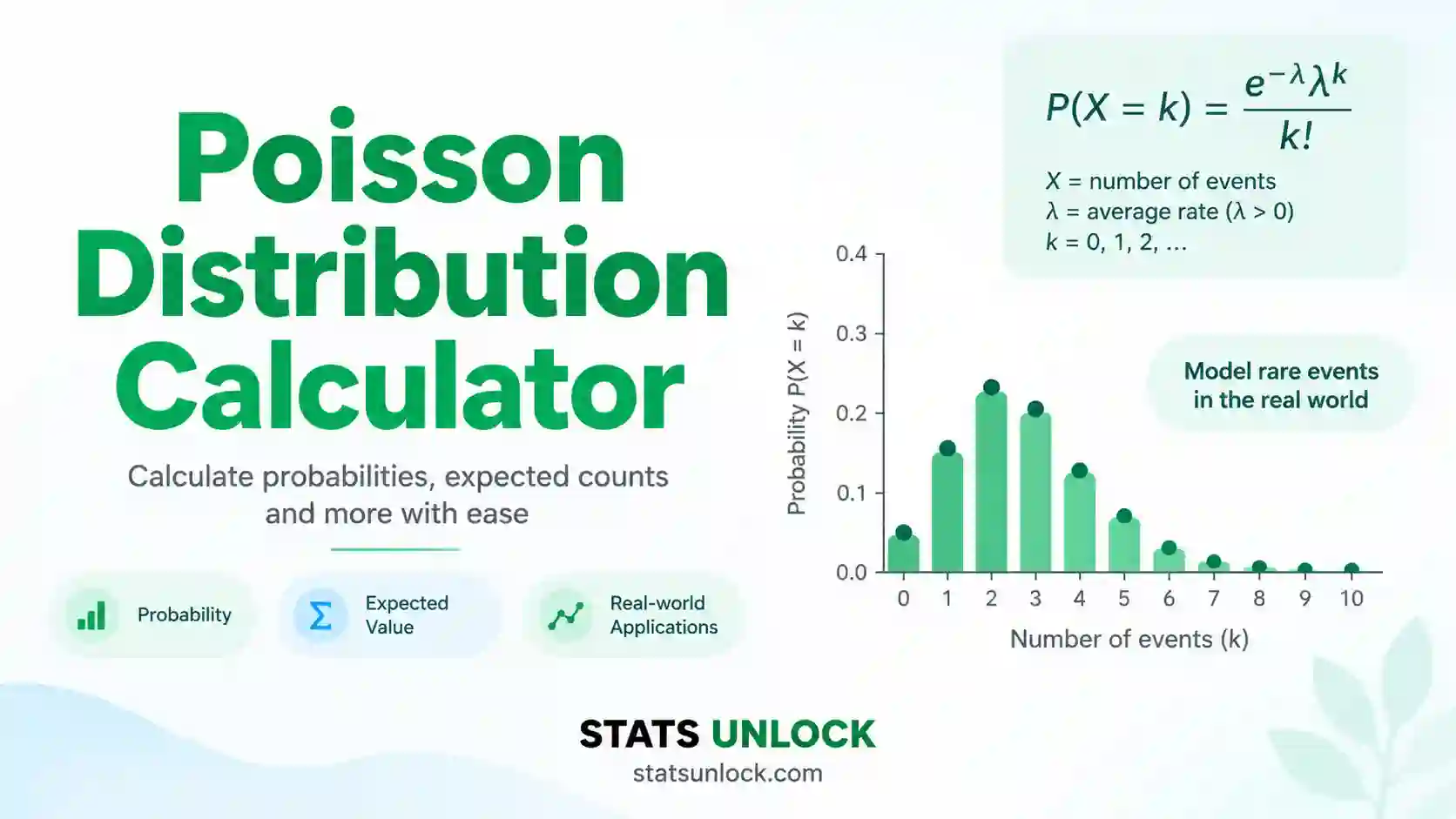
A Poisson distribution calculator finds the chance of seeing exactly x events in a fixed interval when events happen at an average rate λ. The formula is P(X = x) = e−λλx ÷ x!. With λ = 2.15 calls per minute, P(X = 3) = 0.1929 and P(X ≤ 3) = 0.8291. The mean and variance both equal λ.
Rule of thumb: use the Poisson distribution for counts of independent events at a steady rate. If the sample variance is much larger than the mean (variance ÷ mean above about 1.5), the data are overdispersed and a negative binomial model is safer.
🔑 Key Takeaways
- A Poisson distribution calculator needs only one number, λ, the average count per interval.
- The mean and the variance are both equal to λ, so the standard deviation is √λ.
- For the worked example (20 minutes, 43 calls), λ = 2.15 and the exact 95% CI is 1.556 to 2.896.
- A variance-to-mean ratio near 1 supports the Poisson model. Here it is 0.797, dispersion test p = 0.573.
- The Poisson approximates the binomial when n is large and p is small, with λ = np.
📚 1. What Is the Poisson Distribution?
The Poisson distribution is a probability distribution for counts. It tells you how likely it is to see 0, 1, 2, 3 or more events in a fixed interval of time, area, length or volume. Examples are phone calls per minute, cars per hour, typing errors per page, or birds per plot. It is named after the French mathematician Siméon Denis Poisson (1837). The name is pronounced “pwah-SON”.
The whole distribution is controlled by one number, lambda (λ). Lambda is the average number of events per interval. It is also the variance. So a Poisson variable with λ = 4 has a mean of 4, a variance of 4 and a standard deviation of 2.
What it measures: the probability mass function (PMF) gives P(X = x), the chance of exactly x events. The cumulative distribution function (CDF) gives P(X ≤ x), the chance of x events or fewer. The Poisson is discrete: X can only be 0, 1, 2, and so on. There is no continuous Poisson distribution; the continuous partner is the exponential distribution, which models the waiting time between Poisson events.
A worked one-liner: a help desk gets 43 calls in 20 minutes, so λ = 43 ÷ 20 = 2.15 calls per minute. The chance of exactly 3 calls in the next minute is e−2.15 × 2.153 ÷ 3! = 0.1164 × 9.938 ÷ 6 = 0.1929, about 19%.
The four conditions for a Poisson process:
- Events are counted in a fixed interval (one minute, one page, one square metre).
- Events happen independently. One event does not make another more or less likely.
- The average rate λ is constant across the interval.
- Two events cannot happen at exactly the same instant.
Who uses it: call centres plan staff with it, hospitals model patient arrivals, engineers count defects per unit, ecologists test whether animals or plants are randomly spread, insurers model claim counts, physicists count radioactive decays, and web teams model sign-ups or server requests per second.
| Feature | Poisson distribution | Binomial distribution | Normal distribution |
|---|---|---|---|
| Type of data | Counts with no upper limit | Successes out of n fixed trials | Continuous measurements |
| Parameters | λ only | n and p | μ and σ |
| Possible values | 0, 1, 2, … without limit | 0 to n | Any real number |
| Mean | λ | np | μ |
| Variance | λ (equal to the mean) | np(1 − p), smaller than the mean | σ², unrelated to the mean |
| Use when | Rare, independent events in an interval | A fixed number of yes or no trials | Symmetric continuous data, or Poisson with large λ |
🧮 2. Set Up Your Data
Type one count per cell. Each column becomes a cluster. Empty cells are ignored.
🎯 Probability question
📊 3. Results
🧠 4. Interpretation of Results, In Detail
4.1 What lambda (λ) tells you
Lambda is the average number of events in one interval. If λ = 2.15 calls per minute, then over many minutes the typical minute has about two calls. It does not mean every minute has 2.15 calls; counts are always whole numbers. Some minutes have 0 calls, some have 5. Lambda is the long-run average of all those minutes.
Lambda always belongs to an interval. A rate of 2.15 per minute is 129 per hour. If you change the interval, scale λ in the same way: λnew = λ × (new length ÷ old length). Forgetting this step is the most common error in Poisson homework and in real planning work.
4.2 Reading P(X = x), the probability mass function
P(X = x) is the chance of exactly x events. In the worked example P(X = 3) = 0.1929. Say it in words: “In about 19 out of every 100 minutes, the desk gets exactly three calls.” The PMF values for all x add up to 1. The tallest bar is the mode. For a Poisson the mode is the whole-number part of λ, so for λ = 2.15 the most likely count is 2. When λ is a whole number, λ and λ − 1 tie as modes.
4.3 Reading the CDF and the tails
The cumulative distribution function P(X ≤ x) adds the PMF from 0 up to x. P(X ≤ 3) = 0.8291 means 83% of minutes have three calls or fewer. The right tail is the complement. Take care with the wording, because “at least 3” and “more than 3” are different questions:
- At most x: P(X ≤ x) = CDF(x) = 0.8291
- Fewer than x: P(X < x) = CDF(x − 1) = 0.6361
- At least x: P(X ≥ x) = 1 − CDF(x − 1) = 0.3639
- More than x: P(X > x) = 1 − CDF(x) = 0.1709
Because the Poisson is discrete, the “equal to” part matters. For a continuous distribution P(X ≤ 3) and P(X < 3) are the same; for a Poisson they differ by P(X = 3), which here is almost 20 percentage points.
4.4 Mean, variance and standard deviation of a Poisson distribution
The expected value of a Poisson distribution is E(X) = λ, and the variance is Var(X) = λ. So the standard deviation is √λ. For λ = 2.15, the SD is 1.466 calls. This link between mean and variance is the fingerprint of the Poisson. It also means the relative spread, SD ÷ mean = 1 ÷ √λ, shrinks as λ grows. Rare events are noisy; common events are more predictable.
4.5 The estimate λ̂ and its confidence interval
When you paste data, the calculator estimates λ by the sample mean, λ̂ = Σx ÷ n. This is the maximum likelihood estimator (MLE) of the Poisson distribution, and it is also unbiased. The standard error is √(λ̂ ÷ n).
The confidence interval is the exact (Garwood) interval, built from chi-square quantiles. It is not symmetric: the upper arm is longer than the lower arm, because counts cannot go below zero. For the worked example the 95% CI is 1.556 to 2.896 calls per minute. A narrow interval needs a large total count Σx, not just many intervals. Doubling the observation time roughly shrinks the width by √2.
4.6 Is the Poisson a good fit? The dispersion index
The variance-to-mean ratio (the index of dispersion, s² ÷ x̄) should be close to 1. The calculator tests this with D = Σ(x − x̄)² ÷ x̄, which follows a chi-square distribution with n − 1 degrees of freedom if the data are Poisson.
- Ratio near 1, p ≥ 0.05: no evidence against the Poisson. Use it.
- Ratio well above 1, small p: overdispersion. Events cluster (contagion, patchy habitat, mixed groups). Poisson standard errors will be too small. Use a negative binomial or quasi-Poisson model.
- Ratio well below 1, small p: underdispersion. Events are too regular (territorial animals, booked appointments). The Poisson will overstate the spread.
4.7 The chi-square goodness-of-fit test
The goodness-of-fit test compares how many intervals had 0, 1, 2, … events with how many a perfect Poisson would give. Neighbouring bins are merged until every expected count is at least 5 (or the level you pick). The degrees of freedom are bins − 2, because one extra degree is lost for estimating λ from the same data. A large p-value means the observed pattern is consistent with a Poisson. It does not prove the data are Poisson; with small samples the test has little power, so read it together with the dispersion index and Chart 3.
4.8 Decision guide
| What you see | What it means | What to do |
|---|---|---|
| Ratio 0.8 to 1.2, both p ≥ 0.05 | Poisson fits well | Report λ̂, its exact CI, and use the probabilities |
| Ratio above 1.5, dispersion p < 0.05 | Overdispersion | Fit a negative binomial; report the Poisson only as a baseline |
| Many more zeros than expected | Zero inflation | Try a zero-inflated Poisson (ZIP) model |
| Ratio below 0.7, p < 0.05 | Underdispersion, regular spacing | Consider a binomial or a generalized Poisson model |
| Fit test df = 0 | Too few bins after merging | Collect more intervals, or rely on the dispersion test |
| Clusters differ in λ | Rates are not the same | Compare with a Poisson regression or an exact rate test |
4.9 Poisson distribution vs binomial, and vs normal
The binomial counts successes in n fixed trials; the Poisson counts events with no fixed upper limit. When n is large and p is small (a common guide is n ≥ 20 and p ≤ 0.05), Binomial(n, p) is close to Poisson(λ = np). That is the Poisson approximation to the binomial distribution. For example, 1,000 items with a 0.2% defect rate gives λ = 2.
When λ is large (about 20 or more), the Poisson looks like a normal distribution with mean λ and variance λ. Use a continuity correction: P(X ≤ x) ≈ Φ((x + 0.5 − λ) ÷ √λ). For small λ the normal approximation is poor because the Poisson is skewed.
4.10 Common mistakes this calculator prevents
- Mixing up ≥ and >. Every tail is shown separately with its own label.
- Forgetting to rescale λ. The report states the interval each λ belongs to.
- Using the Poisson on overdispersed data. The dispersion test runs automatically.
- Wrong degrees of freedom in the fit test. The calculator uses bins − 2, not bins − 1.
- Symmetric intervals for a rate. The exact Garwood interval is used instead of λ ± 1.96 SE.
- Non-integer or negative counts. These are rejected with a clear message.
✍ 5. How to Write Your Results in Research
When reporting Poisson distribution results in APA format, give four things: the estimated rate λ with its interval and unit of time or space, the confidence interval, a check that the Poisson fits (dispersion index and goodness of fit), and any probability you use for a decision. The five templates below fill in automatically after you run the calculator.
📌 Key conventions for this style
- Italicise statistical symbols such as n, p and χ².
- Report p to three decimals and write p < .001 for very small values.
- State the interval unit every time (per minute, per page, per square metre).
- Name the CI method (exact Garwood) in the Methods section.
📌 Key conventions for this style
- Justify why a Poisson model is suitable before reporting it.
- Report both the dispersion test and the goodness-of-fit test.
- Explain how bins were merged and why the df is bins minus 2.
- Give the software and version.
📌 Key conventions for this style
- Turn probabilities into “out of 100” frequencies.
- Avoid symbols like λ, χ² and p.
- Say what an interval is in everyday words.
- Round to whole percentages.
📌 Key conventions for this style
- Keep one line per heading.
- Put the rate and CI first; tests second.
- Use the same decimals as in your tables.
- Add a footnote for the dispersion index.
📌 Key conventions for this style
- Fix the interval length before data collection.
- State the overdispersion rule and the fallback model in advance.
- Give the minimum expected count for bin merging.
- State alpha and whether tests are two-sided.
∑ 6. Formulas Used
These are the Poisson distribution formulas and equations used by this calculator, from the probability mass function out to the fit tests.
🔀 7. Poisson Distribution Calculation Flowchart, Step by Step
This flowchart shows how the Poisson distribution is calculated, step by step, from raw counts to a checked probability. Every box uses the worked example used in the Excel, R and Python sections: calls to a help desk in 20 one-minute intervals (2, 3, 1, 4, 2, 0, 3, 2, 1, 5, 2, 3, 1, 2, 4, 2, 3, 1, 0, 2).
Check any box yourself: the Excel sheet in Section 9, the R script in Section 10 and the Python script in Section 11 all return these numbers for this dataset.
📝 8. How to Use This Calculator
How to use this Poisson distribution calculator, with the help-desk example as a guide:
- Pick a mode. Choose Fit my count data if you have raw counts, or I already know λ if you only need probabilities.
- Enter your counts. Type comma-separated whole numbers, for example
2, 3, 1, 4, 2, 0, .... Each number is the count in one interval. - Name each cluster. The name box above each textarea is editable, for example Weekday mornings. The name appears in tables, charts and reports.
- Add clusters to compare groups. Press Add cluster. Each cluster gets its own λ, CI and fit tests.
- Or upload a file. On the Upload tab, choose a CSV or Excel file and click the columns you want. Each clicked column becomes its own cluster.
- Try a sample dataset. Ten examples include the classic horse-kick deaths and Rutherford–Geiger decay counts, plus an overdispersed dataset that fails the test.
- Type your probability question. Set x for P(X = x) and the tails, and a to b for a range such as P(1 ≤ X ≤ 4).
- Pick the confidence level and bin rule, then press Calculate Poisson Distribution. Nothing runs until you press it.
- Read the verdict line and the fit checks first. If overdispersion is flagged, treat the Poisson probabilities with caution.
- Check the four charts and export. Section 5 fills five reporting templates, and the buttons save a text report or a print-ready PDF.
📈 9. How to Calculate the Poisson Distribution in Excel
Excel has a built-in Poisson distribution function, POISSON.DIST. It gives both the PMF and the CDF. What catches people out is the tails, the confidence interval for λ, and the goodness-of-fit test, which Excel does not do for you. The steps below rebuild every number on this page for the help-desk example.
=POISSON.DIST(3,B1,FALSE) gives P(X = 3) and =POISSON.DIST(3,B1,TRUE) gives P(X ≤ 3).9.1 The functions you need
| You want | Excel formula | Worked answer |
|---|---|---|
| λ from data | =AVERAGE(A2:A21) | 2.15 |
| P(X = x), the PMF | =POISSON.DIST(3,$E$2,FALSE) | 0.1929 |
| P(X ≤ x), the CDF | =POISSON.DIST(3,$E$2,TRUE) | 0.8291 |
| P(X < x) | =POISSON.DIST(2,$E$2,TRUE) | 0.6361 |
| P(X ≥ x) | =1-POISSON.DIST(2,$E$2,TRUE) | 0.3639 |
| P(X > x) | =1-POISSON.DIST(3,$E$2,TRUE) | 0.1709 |
| P(a ≤ X ≤ b) | =POISSON.DIST(4,$E$2,TRUE)-POISSON.DIST(0,$E$2,TRUE) | 0.8163 |
| Standard deviation | =SQRT($E$2) | 1.4663 |
| Lower 95% CI | =CHISQ.INV(0.025,2*SUM(A2:A21))/(2*COUNT(A2:A21)) | 1.5560 |
| Upper 95% CI | =CHISQ.INV(0.975,2*SUM(A2:A21)+2)/(2*COUNT(A2:A21)) | 2.8960 |
| Dispersion p (two-sided) | =2*MIN(CHISQ.DIST(D,19,TRUE),CHISQ.DIST.RT(D,19)) | 0.5726 |
1-POISSON.DIST(3,λ,TRUE) is P(X > 3), not P(X ≥ 3). For “at least 3” use x − 1 inside the function: 1-POISSON.DIST(2,λ,TRUE). This one slip changes the answer from 0.3639 to 0.1709.9.2 Step by step
1 Put the counts in one column
Type the label Calls in A1 and the 20 counts in A2:A21. One row is one interval. Leave blanks empty; never type 0 for a missing minute.
=COUNT(A2:A21) =SUM(A2:A21)
COUNT returns 20 intervals and SUM returns 43 calls.
2 Estimate lambda and check the variance
Lambda is the average count. Put it in E2 so every later formula can point to it. Then compare the sample variance with it.
=AVERAGE(A2:A21) =VAR.S(A2:A21) =E3/E2
λ = 2.15, variance = 1.7132, ratio = 0.797, close enough to 1.
3 Build the PMF and CDF table
List x = 0 to 8 in G2:G10. In H2 type the PMF formula and in I2 the CDF formula, then fill down.
=POISSON.DIST(G2,$E$2,FALSE) =POISSON.DIST(G2,$E$2,TRUE)
Row x = 3 shows P(X = 3) = 0.1929 and P(X ≤ 3) = 0.8291.
4 Exact confidence interval for lambda
Excel has no Poisson CI function, but the exact interval is two chi-square quantiles.
=CHISQ.INV(0.025,2*E1)/(2*E4) =CHISQ.INV(0.975,2*E1+2)/(2*E4)
With total E1 = 43 and n E4 = 20, the 95% CI is 1.5560 to 2.8960.
5 Goodness-of-fit test
Count observed intervals per bin with COUNTIF, and expected with POISSON.DIST times n. Merge bins so each expected count is at least 5.
=COUNTIF(A2:A21,"<=1") =20*POISSON.DIST(1,$E$2,TRUE) =CHISQ.DIST.RT(0.7394,1)
Bins 0–1, 2 and ≥3 give χ² = 0.7394 with df = 3 − 2 = 1, p = 0.3899.
9.3 The awkward cases
Rescaling lambda. If your rate is per hour and you need per 15 minutes, multiply first: =POISSON.DIST(2,$E$2*15/60,FALSE).
Large lambda. For λ above about 20, a normal approximation is close: =NORM.DIST(x+0.5,λ,SQRT(λ),TRUE). POISSON.DIST itself stays accurate, so use it when you can.
Binomial to Poisson. Compare =BINOM.DIST(2,1000,0.002,FALSE) (0.2709) with =POISSON.DIST(2,2,FALSE) (0.2707). They agree to three decimals.
POISSON(x,mean,cumulative). It gives the same answers as POISSON.DIST and still works for compatibility.9.4 Why your Excel answer might differ from R or Python
| Situation | What happens | Fix |
|---|---|---|
| Decimal x in POISSON.DIST | Excel silently truncates 3.7 to 3 | Counts must be whole numbers; round on purpose |
| P(X ≥ x) vs P(X > x) | Python sf(3) is P(X > 3); R lower.tail=FALSE is also P(X > 3) | Use x − 1 for “at least x” in every program |
| Goodness-of-fit df | R chisq.test(O, p=E/n) uses bins − 1, because it does not know λ was estimated | Recompute p with df = bins − 2, as this page, Excel steps and both scripts do |
| Variance | NumPy var() uses n; Excel VAR.S and R var() use n − 1 | Use np.var(x, ddof=1) |
| Confidence interval | Wald λ ± 1.96√(λ/n) = 1.507 to 2.793 differs from the exact 1.556 to 2.896 | Report the exact interval; R poisson.test gives it |
| Bin merging | Different merging rules give different χ² values | State the rule (E ≥ 5, open last bin) in your methods |
| Tool | P(X = 3) | P(X ≤ 3) | P(X ≥ 3) |
|---|---|---|---|
| Excel / Google Sheets | =POISSON.DIST(3,2.15,FALSE) | =POISSON.DIST(3,2.15,TRUE) | =1-POISSON.DIST(2,2.15,TRUE) |
| R | dpois(3, 2.15) | ppois(3, 2.15) | ppois(2, 2.15, lower.tail = FALSE) |
| Python SciPy | poisson.pmf(3, 2.15) | poisson.cdf(3, 2.15) | poisson.sf(2, 2.15) |
| Answer | 0.1929 | 0.8291 | 0.3639 |
9.5 Charting the Poisson distribution in Excel
- Select the x column and the PMF column (G1:H10).
- Insert → Charts → Clustered Column. Set the gap width to about 30%.
- For an observed vs expected chart, add observed counts as columns and expected counts as a second series, then Change Chart Type → Combo and set expected to Line with Markers.
- For the CDF, select x and the CDF column and choose Insert → Line → Line with Markers.
- Label the x axis “Number of events per interval” and give λ in the title.
Charts 1 to 3 in Section 3 of this page draw these automatically.
9.6 Excel errors you will probably hit
| Excel shows | Why | Fix |
|---|---|---|
#NUM! from POISSON.DIST | x or mean is negative | Both must be 0 or more |
#VALUE! | Text in the x or mean argument | Check the cell is a number, not text |
#NUM! from CHISQ.INV | Degrees of freedom 2T is 0 when there are no events | Set the lower limit to 0 when T = 0 |
| Probability above 1 | Added PMF values of overlapping ranges | Use CDF differences for ranges |
| Answer too small for “at least” | Used x instead of x − 1 in the complement | P(X ≥ x) = 1 − CDF(x − 1) |
| λ looks too low | Missing intervals typed as 0 | Leave missing cells blank so AVERAGE skips them |
| POISSON.DIST not found | Excel 2007 or older | Use POISSON(x,mean,cumulative) |
No Analysis ToolPak is needed for any step above. It has a random number generator with a Poisson option, which must be enabled first under File → Options → Add-ins, but it is only useful for simulation.
📈 10. How to Calculate the Poisson Distribution in R
R has four built-in Poisson functions: dpois for the PMF, ppois for the CDF, qpois for quantiles and rpois for random numbers. The script below uses base R only. It estimates λ, gives the exact CI with poisson.test, runs the dispersion and goodness-of-fit tests with the correct degrees of freedom, prints a plain-English verdict, and saves one 300 dpi figure.
Rscript. Change only the x <- c(...) line to use your own counts.10.1 The complete script
R, base only, saves poisson_fit.png
# ============================================================
# Poisson distribution: fit lambda, test the fit, get probabilities
# StatsUnlock - https://statsunlock.com/poisson-distribution-calculator/
# Base R only. No packages to install.
# ============================================================
set.seed(42)   # nothing random below, kept for reproducibility

# ---- 1. Your data ------------------------------------------
# Replace with your own counts, or read a CSV:
#   x <- read.csv("data.csv")$calls
x <- c(2, 3, 1, 4, 2, 0, 3, 2, 1, 5,
       2, 3, 1, 2, 4, 2, 3, 1, 0, 2)
x <- x[!is.na(x)]                 # drop missing values
label <- "Help desk calls per minute"
x_q <- 3; a <- 1; b <- 4          # probability question
alpha <- 0.05
min_expected <- 5

# ---- 2. Estimate lambda ------------------------------------
n   <- length(x)
tot <- sum(x)
lam <- tot / n                    # MLE = sample mean
s2  <- var(x)                     # var() uses n - 1
se  <- sqrt(lam / n)
ci  <- poisson.test(tot, n, conf.level = 1 - alpha)$conf.int   # exact Garwood CI

# ---- 3. Dispersion test ------------------------------------
D    <- sum((x - lam)^2) / lam
df_d <- n - 1
p_d  <- 2 * min(pchisq(D, df_d), pchisq(D, df_d, lower.tail = FALSE))

# ---- 4. Goodness of fit, bins merged until E >= 5 ----------
poisson_gof <- function(x, lam, min_e) {
  n <- length(x); mx <- max(x)
  lo <- c(); hi <- c(); O <- c(); E <- c()
  start <- 0; e <- 0; o <- 0
  for (k in 0:mx) {
    e <- e + dpois(k, lam) * n
    o <- o + sum(x == k)
    if (e >= min_e && k < mx) {
      lo <- c(lo, start); hi <- c(hi, k); O <- c(O, o); E <- c(E, e)
      start <- k + 1; e <- 0; o <- 0
    }
  }
  lo <- c(lo, start); hi <- c(hi, NA)
  O  <- c(O, sum(x >= start))
  E  <- c(E, ppois(start - 1, lam, lower.tail = FALSE) * n)
  m <- length(E)
  if (E[m] < min_e && m > 1) {
    O[m - 1] <- O[m - 1] + O[m]; E[m - 1] <- E[m - 1] + E[m]; hi[m - 1] <- NA
    lo <- lo[-m]; hi <- hi[-m]; O <- O[-m]; E <- E[-m]
  }
  chi <- sum((O - E)^2 / E)
  df  <- length(E) - 2            # minus 1 for estimating lambda
  p   <- if (df > 0) pchisq(chi, df, lower.tail = FALSE) else NA
  list(table = data.frame(from = lo, to = hi, observed = O, expected = round(E, 3)),
       chi = chi, df = df, p = p)
}
g <- poisson_gof(x, lam, min_expected)

# ---- 5. Print everything -----------------------------------
cat(label, "\n")
cat(sprintf("n = %d, total = %d, lambda = %.4f, variance = %.4f\n", n, tot, lam, s2))
cat(sprintf("SD of Poisson = %.4f, SE of lambda = %.4f\n", sqrt(lam), se))
cat(sprintf("%d%% exact CI for lambda = %.4f to %.4f\n", round((1 - alpha) * 100), ci[1], ci[2]))
cat(sprintf("variance / mean = %.4f, D = %.4f, df = %d, p = %.4f\n", s2 / lam, D, df_d, p_d))
print(g$table)
cat(sprintf("goodness of fit chi-square(%d) = %.4f, p = %.4f\n", g$df, g$chi, g$p))
cat(sprintf("P(X = %d)  = %.4f\n", x_q, dpois(x_q, lam)))
cat(sprintf("P(X <= %d) = %.4f\n", x_q, ppois(x_q, lam)))
cat(sprintf("P(X < %d)  = %.4f\n", x_q, ppois(x_q - 1, lam)))
cat(sprintf("P(X >= %d) = %.4f\n", x_q, ppois(x_q - 1, lam, lower.tail = FALSE)))
cat(sprintf("P(X > %d)  = %.4f\n", x_q, ppois(x_q, lam, lower.tail = FALSE)))
cat(sprintf("P(%d <= X <= %d) = %.4f\n", a, b, ppois(b, lam) - ppois(a - 1, lam)))
ok <- p_d >= 0.05 && (is.na(g$p) || g$p >= 0.05)
cat("Verdict:", if (ok) "the Poisson distribution fits these counts.\n"
    else "the Poisson does not fit well; check for overdispersion.\n")

# ---- 6. One figure: observed vs expected -------------------
k   <- 0:max(max(x), ceiling(lam + 4 * sqrt(lam)))
obs <- sapply(k, function(v) sum(x == v))
ex  <- dpois(k, lam) * n
png("poisson_fit.png", width = 7, height = 4.2, units = "in", res = 300)
par(mar = c(4.5, 4.5, 3, 1))
mids <- barplot(obs, names.arg = k, col = "#60a5fa", border = "#1d4ed8",
                ylim = c(0, max(obs, ex) * 1.2),
                xlab = "Number of events per interval (x)",
                ylab = "Number of intervals", main = label)
lines(mids, ex, type = "b", pch = 19, col = "#c2410c", lwd = 2)
legend("topright", bty = "n", fill = c("#60a5fa", NA), border = c("#1d4ed8", NA),
       lty = c(NA, 1), pch = c(NA, 19), col = c(NA, "#c2410c"),
       legend = c("Observed intervals", sprintf("Poisson expected, lambda = %.2f", lam)))
dev.off()
cat("Saved poisson_fit.png\n")
10.2 What each part does
| Line or function | What it does and why |
|---|---|
| x[!is.na(x)] | Drops missing intervals so they do not count as zero |
| lam <- tot / n | The maximum likelihood estimate of λ, the sample mean |
| poisson.test(tot, n) | Exact Garwood CI for the rate; the second argument is the time base n |
| pchisq(D, n - 1) | Dispersion test; two-sided so it catches under- and overdispersion |
| poisson_gof() | Merges bins until E ≥ 5, adds an open last bin, uses df = bins − 2 |
| dpois / ppois | PMF and CDF; lower.tail = FALSE gives P(X > x) |
| png(..., res = 300) | Saves a 300 dpi figure for a paper or thesis |
10.3 What the figure shows
Blue bars are how many minutes had 0, 1, 2, … calls. The orange line is how many a perfect Poisson with λ = 2.15 would give. The bars follow the line closely, with slightly more 2s and fewer 0s and 1s than expected, which matches the non-significant fit test (p = 0.390).
10.4 Problems and fixes
| Problem | Fix |
|---|---|
chisq.test gives a different p-value | It uses bins − 1 df. Use pchisq(stat, bins - 2, lower.tail = FALSE) |
| Warning: Chi-squared approximation may be incorrect | Some expected counts are below 5; merge bins as the script does |
| Variance far above the mean | Fit MASS::glm.nb(x ~ 1) instead |
poisson.test error: x must be integer | Your counts contain decimals; they are not Poisson counts |
10.5 One-liners
| Task | R code |
|---|---|
| P(X = 3) | dpois(3, 2.15) |
| P(X ≤ 3) | ppois(3, 2.15) |
| P(X ≥ 3) | 1 - ppois(2, 2.15) |
| Poisson distribution table 0 to 10 | round(dpois(0:10, 2.15), 4) |
| 95th percentile | qpois(0.95, 2.15) |
| Simulate 1000 counts | rpois(1000, 2.15) |
| Poisson regression | glm(y ~ x, family = poisson) |
📈 11. How to Calculate the Poisson Distribution in Python
In Python the Poisson distribution lives in scipy.stats.poisson. The script below matches the R script number for number: λ, the exact CI, the dispersion test, the goodness-of-fit test with df = bins − 2, every tail probability and a 300 dpi figure.
x = np.array([...]) line. Install once with pip install numpy scipy matplotlib pandas.11.1 The complete script
Python 3, saves poisson_fit.png
# ============================================================
# Poisson distribution: fit lambda, test the fit, get probabilities
# StatsUnlock - https://statsunlock.com/poisson-distribution-calculator/
# pip install numpy scipy matplotlib pandas
# ============================================================
import numpy as np
from scipy import stats
import matplotlib
matplotlib.use("Agg")
import matplotlib.pyplot as plt

np.random.seed(42)  # nothing random below, kept for reproducibility

# ---- 1. Your data ------------------------------------------
# Replace with your own counts, or read a CSV:
#   import pandas as pd
#   x = pd.read_csv("data.csv")["calls"].dropna().astype(int).to_numpy()
x = np.array([2, 3, 1, 4, 2, 0, 3, 2, 1, 5,
              2, 3, 1, 2, 4, 2, 3, 1, 0, 2])
label = "Help desk calls per minute"
x_q, a, b = 3, 1, 4          # probability question
alpha = 0.05
min_expected = 5

x = x[~np.isnan(x)] if x.dtype.kind == "f" else x   # drop missing values

# ---- 2. Estimate lambda ------------------------------------
n = len(x)
T = x.sum()
lam = T / n                                   # MLE = sample mean
s2 = x.var(ddof=1)                            # sample variance, n - 1
se = np.sqrt(lam / n)
lo = stats.chi2.ppf(alpha / 2, 2 * T) / (2 * n) if T > 0 else 0.0
hi = stats.chi2.ppf(1 - alpha / 2, 2 * T + 2) / (2 * n)

# ---- 3. Dispersion test ------------------------------------
D = ((x - lam) ** 2).sum() / lam
df_d = n - 1
p_d = 2 * min(stats.chi2.cdf(D, df_d), stats.chi2.sf(D, df_d))

# ---- 4. Goodness of fit, bins merged until E >= 5 ----------
def poisson_gof(x, lam, min_e):
    n, mx = len(x), x.max()
    bins, start, E, O = [], 0, 0.0, 0
    for k in range(mx + 1):
        E += stats.poisson.pmf(k, lam) * n
        O += (x == k).sum()
        if E >= min_e and k < mx:
            bins.append([start, k, O, E]); start, E, O = k + 1, 0.0, 0
    bins.append([start, None, (x >= start).sum(), stats.poisson.sf(start - 1, lam) * n])
    if bins[-1][3] < min_e and len(bins) > 1:
        last = bins.pop()
        bins[-1][1] = None; bins[-1][2] += last[2]; bins[-1][3] += last[3]
    chi = sum((o - e) ** 2 / e for _, _, o, e in bins)
    df = len(bins) - 2                        # minus 1 for estimating lambda
    p = stats.chi2.sf(chi, df) if df > 0 else float("nan")
    return bins, chi, df, p

bins, chi, df_g, p_g = poisson_gof(x, lam, min_expected)

# ---- 5. Probabilities --------------------------------------
P = stats.poisson
print(f"{label}")
print(f"n = {n}, total = {T}, lambda = {lam:.4f}, variance = {s2:.4f}")
print(f"SD of Poisson = {np.sqrt(lam):.4f}, SE of lambda = {se:.4f}")
print(f"{int((1-alpha)*100)}% exact CI for lambda = {lo:.4f} to {hi:.4f}")
print(f"variance / mean = {s2/lam:.4f}, D = {D:.4f}, df = {df_d}, p = {p_d:.4f}")
for lo_k, hi_k, o, e in bins:
    tag = f"{lo_k}" if hi_k == lo_k else (f">={lo_k}" if hi_k is None else f"{lo_k}-{hi_k}")
    print(f"  bin {tag:>5}: observed {o:3d}, expected {e:7.3f}")
print(f"goodness of fit chi-square({df_g}) = {chi:.4f}, p = {p_g:.4f}")
print(f"P(X = {x_q})  = {P.pmf(x_q, lam):.4f}")
print(f"P(X <= {x_q}) = {P.cdf(x_q, lam):.4f}")
print(f"P(X < {x_q})  = {P.cdf(x_q - 1, lam):.4f}")
print(f"P(X >= {x_q}) = {P.sf(x_q - 1, lam):.4f}")
print(f"P(X > {x_q})  = {P.sf(x_q, lam):.4f}   # scipy sf(k) is P(X > k)")
print(f"P({a} <= X <= {b}) = {P.cdf(b, lam) - P.cdf(a - 1, lam):.4f}")
ok = p_d >= 0.05 and (np.isnan(p_g) or p_g >= 0.05)
print("Verdict:", "the Poisson distribution fits these counts." if ok
      else "the Poisson does not fit well; check for overdispersion.")

# ---- 6. One figure: observed vs expected -------------------
k = np.arange(0, max(x.max(), int(lam + 4 * np.sqrt(lam))) + 1)
obs = np.array([(x == v).sum() for v in k])
exp_ = P.pmf(k, lam) * n
fig, ax = plt.subplots(figsize=(7, 4.2))
ax.bar(k, obs, color="#60a5fa", edgecolor="#1d4ed8", label="Observed intervals")
ax.plot(k, exp_, "o-", color="#c2410c", lw=2, label=f"Poisson expected, lambda = {lam:.2f}")
ax.set_xlabel("Number of events per interval (x)")
ax.set_ylabel("Number of intervals")
ax.set_title(label)
ax.set_xticks(k)
ax.legend(frameon=False)
fig.tight_layout()
fig.savefig("poisson_fit.png", dpi=300)
print("Saved poisson_fit.png")
Output for the worked example: n = 20, total = 43, lambda = 2.1500, 95% CI 1.5560 to 2.8960, D = 15.1395 (df 19, p = 0.5726), goodness of fit χ²(1) = 0.7394, p = 0.3899, P(X = 3) = 0.1929, P(X ≤ 3) = 0.8291, P(X ≥ 3) = 0.3639, P(1 ≤ X ≤ 4) = 0.8163.
11.2 What each part does
| Line or function | What it does and why |
|---|---|
| x.var(ddof=1) | Sample variance with n − 1; the NumPy default ddof=0 would give 1.6275 |
| stats.chi2.ppf(...) | Chi-square quantiles for the exact Garwood CI |
| poisson.sf(k, lam) | P(X > k). For P(X ≥ k) pass k − 1 |
| poisson_gof() | Same bin-merging rule as R and this page; df = bins − 2 |
| fig.savefig(dpi=300) | Saves the figure at print quality |
11.3 What the figure shows
The figure is the same as the R version: observed minutes as blue bars, expected Poisson counts as an orange line. Use it as the main figure when you report a Poisson fit.
11.4 Problems and fixes
| Problem | Fix |
|---|---|
scipy.stats.chisquare p differs | Pass ddof=1 so df = bins − 2 |
| Expected and observed totals differ | Use an open last bin with sf, as the script does |
poisson.pmf(2.5, lam) returns 0 | Non-integer x has zero probability; counts must be whole numbers |
| Overdispersion flagged | Use statsmodels NegativeBinomial or GLM with a negative binomial family |
11.5 One-liners
| Task | Python code |
|---|---|
| P(X = 3) | poisson.pmf(3, 2.15) |
| P(X ≤ 3) | poisson.cdf(3, 2.15) |
| P(X ≥ 3) | poisson.sf(2, 2.15) |
| Mean, variance, skew, kurtosis | poisson.stats(2.15, moments="mvsk") |
| Poisson distribution sample | np.random.default_rng(42).poisson(2.15, 1000) |
| 95th percentile | poisson.ppf(0.95, 2.15) |
📋 12. Reference Tables
12.1 Poisson distribution table, P(X = x)
| x | λ = 0.5 | λ = 1 | λ = 2 | λ = 3 | λ = 4 | λ = 5 | λ = 8 | λ = 10 |
|---|---|---|---|---|---|---|---|---|
| 0 | 0.6065 | 0.3679 | 0.1353 | 0.0498 | 0.0183 | 0.0067 | 0.0003 | 0.0000 |
| 1 | 0.3033 | 0.3679 | 0.2707 | 0.1494 | 0.0733 | 0.0337 | 0.0027 | 0.0005 |
| 2 | 0.0758 | 0.1839 | 0.2707 | 0.2240 | 0.1465 | 0.0842 | 0.0107 | 0.0023 |
| 3 | 0.0126 | 0.0613 | 0.1804 | 0.2240 | 0.1954 | 0.1404 | 0.0286 | 0.0076 |
| 4 | 0.0016 | 0.0153 | 0.0902 | 0.1680 | 0.1954 | 0.1755 | 0.0573 | 0.0189 |
| 5 | 0.0002 | 0.0031 | 0.0361 | 0.1008 | 0.1563 | 0.1755 | 0.0916 | 0.0378 |
| 6 | 0.0000 | 0.0005 | 0.0120 | 0.0504 | 0.1042 | 0.1462 | 0.1221 | 0.0631 |
| 7 | 0.0000 | 0.0001 | 0.0034 | 0.0216 | 0.0595 | 0.1044 | 0.1396 | 0.0901 |
| 8 | 0.0000 | 0.0000 | 0.0009 | 0.0081 | 0.0298 | 0.0653 | 0.1396 | 0.1126 |
| 9 | 0.0000 | 0.0000 | 0.0002 | 0.0027 | 0.0132 | 0.0363 | 0.1241 | 0.1251 |
| 10 | 0.0000 | 0.0000 | 0.0000 | 0.0008 | 0.0053 | 0.0181 | 0.0993 | 0.1251 |
| 11 | 0.0000 | 0.0000 | 0.0000 | 0.0002 | 0.0019 | 0.0082 | 0.0722 | 0.1137 |
| 12 | 0.0000 | 0.0000 | 0.0000 | 0.0001 | 0.0006 | 0.0034 | 0.0481 | 0.0948 |
| 13 | 0.0000 | 0.0000 | 0.0000 | 0.0000 | 0.0002 | 0.0013 | 0.0296 | 0.0729 |
| 14 | 0.0000 | 0.0000 | 0.0000 | 0.0000 | 0.0001 | 0.0005 | 0.0169 | 0.0521 |
| 15 | 0.0000 | 0.0000 | 0.0000 | 0.0000 | 0.0000 | 0.0002 | 0.0090 | 0.0347 |
Conclusion: read down a column for your λ. The largest value in each column sits at x = λ (or λ − 1 and λ tied when λ is a whole number).
12.2 Cumulative Poisson probability table, P(X ≤ x)
| x | λ = 0.5 | λ = 1 | λ = 2 | λ = 3 | λ = 4 | λ = 5 | λ = 8 | λ = 10 |
|---|---|---|---|---|---|---|---|---|
| 0 | 0.6065 | 0.3679 | 0.1353 | 0.0498 | 0.0183 | 0.0067 | 0.0003 | 0.0000 |
| 1 | 0.9098 | 0.7358 | 0.4060 | 0.1991 | 0.0916 | 0.0404 | 0.0030 | 0.0005 |
| 2 | 0.9856 | 0.9197 | 0.6767 | 0.4232 | 0.2381 | 0.1247 | 0.0138 | 0.0028 |
| 3 | 0.9982 | 0.9810 | 0.8571 | 0.6472 | 0.4335 | 0.2650 | 0.0424 | 0.0103 |
| 4 | 0.9998 | 0.9963 | 0.9473 | 0.8153 | 0.6288 | 0.4405 | 0.0996 | 0.0293 |
| 5 | 1.0000 | 0.9994 | 0.9834 | 0.9161 | 0.7851 | 0.6160 | 0.1912 | 0.0671 |
| 6 | 1.0000 | 0.9999 | 0.9955 | 0.9665 | 0.8893 | 0.7622 | 0.3134 | 0.1301 |
| 7 | 1.0000 | 1.0000 | 0.9989 | 0.9881 | 0.9489 | 0.8666 | 0.4530 | 0.2202 |
| 8 | 1.0000 | 1.0000 | 0.9998 | 0.9962 | 0.9786 | 0.9319 | 0.5925 | 0.3328 |
| 9 | 1.0000 | 1.0000 | 1.0000 | 0.9989 | 0.9919 | 0.9682 | 0.7166 | 0.4579 |
| 10 | 1.0000 | 1.0000 | 1.0000 | 0.9997 | 0.9972 | 0.9863 | 0.8159 | 0.5830 |
| 11 | 1.0000 | 1.0000 | 1.0000 | 0.9999 | 0.9991 | 0.9945 | 0.8881 | 0.6968 |
| 12 | 1.0000 | 1.0000 | 1.0000 | 1.0000 | 0.9997 | 0.9980 | 0.9362 | 0.7916 |
| 13 | 1.0000 | 1.0000 | 1.0000 | 1.0000 | 0.9999 | 0.9993 | 0.9658 | 0.8645 |
| 14 | 1.0000 | 1.0000 | 1.0000 | 1.0000 | 1.0000 | 0.9998 | 0.9827 | 0.9165 |
| 15 | 1.0000 | 1.0000 | 1.0000 | 1.0000 | 1.0000 | 0.9999 | 0.9918 | 0.9513 |
Conclusion: P(X ≥ x) = 1 minus the value one row above. For λ = 2, P(X ≥ 4) = 1 − 0.8571 = 0.1429.
12.3 Mean, variance, standard deviation and shape by λ
| λ | Mean | Variance | SD | Skewness | P(X = 0) | 95th percentile |
|---|---|---|---|---|---|---|
| 0.5 | 0.5 | 0.5 | 0.707 | 1.414 | 0.6065 | 2 |
| 1 | 1 | 1 | 1.000 | 1.000 | 0.3679 | 3 |
| 2 | 2 | 2 | 1.414 | 0.707 | 0.1353 | 5 |
| 5 | 5 | 5 | 2.236 | 0.447 | 0.0067 | 9 |
| 10 | 10 | 10 | 3.162 | 0.316 | 0.0000 | 15 |
| 20 | 20 | 20 | 4.472 | 0.224 | 0.0000 | 28 |
| 50 | 50 | 50 | 7.071 | 0.141 | 0.0000 | 62 |
| 100 | 100 | 100 | 10.000 | 0.100 | 0.0000 | 117 |
Conclusion: skewness falls as λ rises. Above λ ≈ 20 the Poisson is nearly symmetric and a normal approximation works well.
12.4 Poisson approximation to the binomial
| n | p | λ = np | Binomial P(X = 2) | Poisson P(X = 2) | Difference | Verdict |
|---|---|---|---|---|---|---|
| 10 | 0.2 | 2 | 0.3020 | 0.2707 | 0.0313 | Poor |
| 20 | 0.1 | 2 | 0.2852 | 0.2707 | 0.0145 | Fair |
| 50 | 0.04 | 2 | 0.2762 | 0.2707 | 0.0056 | Fair |
| 100 | 0.02 | 2 | 0.2734 | 0.2707 | 0.0027 | Fair |
| 1000 | 0.002 | 2 | 0.2709 | 0.2707 | 0.0003 | Excellent |
Conclusion: with λ held at 2, the approximation improves as n grows and p shrinks. Use it when n ≥ 20 and p ≤ 0.05.
12.5 Chi-square critical values for the fit and dispersion tests
| df | α = 0.10 | α = 0.05 | α = 0.01 |
|---|---|---|---|
| 1 | 2.706 | 3.841 | 6.635 |
| 2 | 4.605 | 5.991 | 9.210 |
| 3 | 6.251 | 7.815 | 11.345 |
| 4 | 7.779 | 9.488 | 13.277 |
| 5 | 9.236 | 11.070 | 15.086 |
| 6 | 10.645 | 12.592 | 16.812 |
| 8 | 13.362 | 15.507 | 20.090 |
| 10 | 15.987 | 18.307 | 23.209 |
| 15 | 22.307 | 24.996 | 30.578 |
| 19 | 27.204 | 30.144 | 36.191 |
| 20 | 28.412 | 31.410 | 37.566 |
| 30 | 40.256 | 43.773 | 50.892 |
Conclusion: the worked goodness-of-fit χ² of 0.739 on 1 df is far below 3.841, so the Poisson is not rejected.
12.6 Variance-to-mean ratio guide
| Ratio s² ÷ x̄ | Pattern | Typical cause | Model to use |
|---|---|---|---|
| below 0.7 | Underdispersed | Regular spacing, territories, booked slots | Binomial or generalized Poisson |
| 0.7 to 1.3 | Poisson-like | Random, independent events | Poisson |
| 1.3 to 2 | Mild overdispersion | Some clustering or rate changes | Test it; quasi-Poisson if significant |
| above 2 | Overdispersed | Contagion, patchy habitat, mixed groups | Negative binomial |
Conclusion: these bands are guides only. Always confirm with the dispersion test, whose power depends on n.
📈 13. Example Results
Eight worked examples of the Poisson distribution, from the textbook case to a clear failure. Each shows the observed counts against a perfect Poisson.
Prussian horse-kick deaths (Bortkiewicz)
The dataset that made the Poisson distribution famous.
Deaths from horse kicks in 10 Prussian army corps over 20 years: 200 corps-years, 122 deaths.
| n | λ̂ | 95% CI | s² ÷ x̄ | Dispersion p | GOF χ² (df), p |
|---|---|---|---|---|---|
| 200 | 0.610 | 0.507 to 0.728 | 1.002 | 0.961 | 0.06 (1), 0.802 |
What it means: The rate is 0.61 deaths per corps-year, and the variance is almost exactly the mean (1.002). The fit is excellent (p = 0.802). Rare, independent events at a steady rate are exactly what a Poisson process describes.
How to write it: Deaths per corps-year followed a Poisson distribution, λ = 0.61, 95% CI [0.51, 0.73], χ²(1) = 0.06, p = 0.802.
Parasites per fish
A strong rejection: the counts are far too spread out.
Parasite counts on 40 fish from one lake. A few fish carry many parasites and many carry none.
| n | λ̂ | 95% CI | s² ÷ x̄ | Dispersion p | GOF χ² (df), p |
|---|---|---|---|---|---|
| 40 | 3.250 | 2.715 to 3.859 | 3.531 | < .001 | 14.75 (3), 0.002 |
What it means: The variance is 3.5 times the mean. Both tests reject the Poisson (dispersion p < .001, fit p = 0.002). Parasites aggregate on a few hosts, so a negative binomial model is needed.
How to write it: Counts were strongly overdispersed (s²/x̄ = 3.53, χ²(39) = 137.7, p < .001), so a negative binomial model was used.
Bird nests per quadrat
Close to the line: report it honestly.
36 quadrats of 10 m × 10 m in a grassland, counting active nests.
| n | λ̂ | 95% CI | s² ÷ x̄ | Dispersion p | GOF χ² (df), p |
|---|---|---|---|---|---|
| 36 | 2.306 | 1.836 to 2.858 | 1.507 | 0.055 | 0.34 (2), 0.844 |
What it means: The ratio is 1.51 and the dispersion test gives p = 0.055, just above 0.05. The shape test passes (p = 0.844). There is a hint of clumping. Say so, and check the result with a negative binomial fit before relying on tail probabilities.
How to write it: Nest counts showed mild, non-significant overdispersion (s²/x̄ = 1.51, χ²(35) = 52.76, p = 0.055).
Help desk calls per minute
The worked example used everywhere on this page.
20 one-minute intervals, 43 calls. Question: how often do we get 3 calls in a minute?
| n | λ̂ | 95% CI | s² ÷ x̄ | Dispersion p | GOF χ² (df), p |
|---|---|---|---|---|---|
| 20 | 2.150 | 1.556 to 2.896 | 0.797 | 0.573 | 0.74 (1), 0.390 |
What it means: No evidence against the Poisson (dispersion p = 0.573, fit p = 0.390). Exactly three calls happen in about 19% of minutes; three or more in about 36%.
How to write it: Calls per minute followed a Poisson distribution, λ = 2.15, 95% CI [1.56, 2.90]; s²/x̄ = 0.80, χ²(19) = 15.14, p = .573.
Workplace incidents per month
Only six months of data: the CI is wide.
A small site recorded 1, 0, 2, 1, 3, 1 incidents over six months.
| n | λ̂ | 95% CI | s² ÷ x̄ | Dispersion p | GOF χ² (df), p |
|---|---|---|---|---|---|
| 6 | 1.333 | 0.576 to 2.627 | 0.800 | 0.901 | n/a |
What it means: The best estimate is 1.33 incidents per month, but the 95% CI runs from 0.58 to 2.63, a four-fold range. The goodness-of-fit test is not possible (too few bins). Do not claim the process is Poisson; collect more months.
How to write it: The incident rate was 1.33 per month (95% CI [0.58, 2.63], n = 6); the sample was too small to test the Poisson assumption.
Calls to a national hotline, 3,000 intervals
Huge n makes a tiny departure significant.
3,000 five-minute intervals from a national hotline.
| n | λ̂ | 95% CI | s² ÷ x̄ | Dispersion p | GOF χ² (df), p |
|---|---|---|---|---|---|
| 3000 | 4.031 | 3.960 to 4.104 | 1.116 | < .001 | 30.18 (10), < .001 |
What it means: The ratio is only 1.12, yet both tests are significant because n is so large. The Poisson still predicts the probabilities well (Chart shows near-perfect agreement). For planning, the Poisson is good enough; for standard errors, use a quasi-Poisson correction.
How to write it: Although overdispersion was statistically significant (s²/x̄ = 1.12, p < .001), its size was small, and Poisson probabilities were used with quasi-Poisson standard errors.
Beetles per trap, many empty traps
Too many zeros: a zero-inflated process.
60 pitfall traps; about a third were in dry soil where beetles never occur.
| n | λ̂ | 95% CI | s² ÷ x̄ | Dispersion p | GOF χ² (df), p |
|---|---|---|---|---|---|
| 60 | 2.283 | 1.917 to 2.699 | 2.065 | < .001 | 53.55 (3), < .001 |
What it means: There are 21 empty traps where the Poisson expects about 6. The fit fails badly (p < .001). Two processes are mixed: habitat decides if beetles can be present, and a Poisson process gives the count where they are. Use a zero-inflated Poisson model.
How to write it: Counts contained excess zeros (21 observed vs 6.1 expected; χ²(3) = 53.6, p < .001), so a zero-inflated Poisson model was fitted.
Staffing an emergency room
Using a known λ for a capacity decision.
An ER averages λ = 6 arrivals per hour. Staff can handle 9 per hour. How often is capacity exceeded?
| λ | P(X ≤ 9) | P(X ≥ 10) | Hours per 24 over capacity | Capacity for 95% of hours | for 99% |
|---|---|---|---|---|---|
| 6 | 0.9161 | 0.0839 | 2.01 | 10 | 12 |
What it means: capacity is exceeded in about 8.4% of hours, roughly 2.0 hours a day. Staffing for 10 per hour covers 95% of hours; 12 per hour covers 99%.
How to write it: Assuming Poisson arrivals with λ = 6 per hour, the probability of 10 or more arrivals in an hour was 0.084.
🧪 14. Data Collection Protocol
Study design: count the number of events in many equal, non-overlapping intervals of time or space, with the same conditions in every interval. Each interval gives one whole-number count.
- Define the event exactly. Write down what counts as one event (one call answered, one defect over 1 mm, one nest with eggs). Vague rules add noise that looks like overdispersion.
- Fix the interval length before you start. One minute, one page, one 10 m × 10 m quadrat. Every interval must be the same size, or you need a rate model with an offset.
- Keep conditions steady. Do not mix busy and quiet hours in one sample. If the rate changes with time of day, record it as a separate cluster.
- Choose intervals at random or systematically. Picking only “interesting” intervals biases λ upward.
- Make the intervals independent. Leave gaps between intervals if events can trigger each other, such as repeat calls.
- Record zeros. An interval with no events is a real observation with the value 0. Leaving zeros out inflates λ and wrecks the fit test.
- Record missing intervals as blank, never as 0. A broken counter is not a zero count.
- Collect enough intervals. Aim for at least 30 intervals, and a total count T of at least 30, so the CI is useful and the fit test has several bins.
- Log the conditions. Date, time, observer and any unusual event, so you can explain outliers later.
- Plan the model check. Decide now that you will use the dispersion test and switch to a negative binomial model if p < 0.05.
| interval_id | date | start_time | length_min | cluster | count |
|---|---|---|---|---|---|
| 1 | 2026-03-02 | 09:00 | 1 | Weekday | 2 |
| 2 | 2026-03-02 | 09:05 | 1 | Weekday | 3 |
| 3 | 2026-03-02 | 09:10 | 1 | Weekday | 0 |
Minimum sample: 30 or more intervals and a total count of 30 or more. With fewer, report λ and its exact CI but treat the fit tests as weak.
Pre-registration line: “Counts per fixed interval will be modelled as Poisson; if the index of dispersion test gives p < .05, a negative binomial model will be used instead.”
Common mistakes: unequal intervals, dropping zero counts, typing 0 for missing data, pooling different time periods, and counting the same event twice across neighbouring intervals.
🎯 15. When to Use the Poisson Distribution
This free Poisson distribution calculator is designed for students, teachers, analysts and researchers who work with counts of random events.
- You count events in fixed intervals of time or space
- Events happen one at a time and independently
- The average rate is steady
- There is no fixed maximum number of events
- The variance is about equal to the mean
- There is a fixed number of trials (use the binomial)
- The variance is much larger than the mean (use a negative binomial)
- There are far more zeros than expected (use a zero-inflated model)
- You measure time between events (use the exponential)
- The data are measurements, not counts (use the normal)
Four examples of the Poisson distribution:
- Operations: a call centre averages 2.15 calls per minute; what is the chance of 5 or more in one minute?
- Health care: an emergency room averages 6 arrivals per hour; how many nurses cover 95% of hours?
- Quality control: 0.8 defects per circuit board; what share of boards will be defect-free? P(X = 0) = e−0.8 = 0.449.
- Ecology: are nests spread at random across quadrats, or clumped? The dispersion test answers this.
Design guidance: choose an interval long enough that most intervals have at least one event (λ around 1 to 10 is easiest to work with), but short enough that the rate stays steady within it.
🔧 16. Troubleshooting and Common Errors
“Counts must be whole numbers” message
Cause: a decimal or negative value, often a rate or average. Fix: enter raw counts per interval. If you only have a rate, switch to I already know λ.
Fit test shows df = 0 or “not available”
Cause: after merging bins so each expected count is at least 5, fewer than 3 bins remain. Fix: collect more intervals, pick the lenient 3 or 1 rule, or rely on the dispersion test.
Variance is much larger than the mean
Cause: events cluster, or the rate differs between intervals. Fix: split the data into clusters by time or place, or fit a negative binomial model.
My answer for “at least x” is too small
Cause: you used 1 − CDF(x), which is P(X > x). Fix: P(X ≥ x) = 1 − CDF(x − 1). This calculator shows both.
R chisq.test gives a different p-value
Cause: R uses bins − 1 degrees of freedom. Fix: recompute with df = bins − 2, because λ was estimated from the data.
Python and Excel variance disagree
Cause: NumPy's default divides by n. Fix: use np.var(x, ddof=1) to match VAR.S.
Many more zeros than expected
Cause: two processes, for example sites that can never have the event. Fix: use a zero-inflated Poisson model, and look at Chart 3.
The CSV upload shows no columns
Cause: the columns contain text or the first row is not a header. Fix: keep one header row and numbers below it; only numeric columns are offered.
The confidence interval looks lopsided
Cause: this is correct. The exact interval is not symmetric because counts cannot go below zero. Fix: nothing to fix; report it as it is.
Charts look empty for very large λ
Cause: with λ in the hundreds each single probability is tiny. Fix: read the CDF chart, or rescale the interval so λ is smaller.
⚖ 17. Assumptions and Limitations
17.1 Assumptions of the Poisson distribution
- Counts in fixed intervals. Check: all intervals are equal. If broken: λ mixes different exposures and is biased toward the longer intervals.
- Independence. Check: plot counts in time order and look for runs. If broken (contagion): variance is inflated, SEs are too small, p-values too small.
- Constant rate. Check: compare λ across clusters or halves of the data. If broken: overdispersion appears, and tail probabilities are underestimated.
- No simultaneous events. Check: events are recorded one by one. If broken (batches): counts jump in groups and variance is too large.
- Mean equals variance. Check: the dispersion test. If broken: overdispersion makes the Poisson CI too narrow; underdispersion makes it too wide.
17.2 Limitations of this calculator
- It fits one λ per cluster. To model λ as a function of predictors, use Poisson regression (a GLM).
- It does not fit a negative binomial or zero-inflated model. It flags the need for one.
- The goodness-of-fit test has low power with fewer than about 30 intervals. Use a likelihood-based test or simulation for small samples.
- It does not compare two rates formally. Use an exact conditional test or Poisson regression.
- It cannot fix biased sampling. A precise λ from unrepresentative intervals is still wrong.
🏁 18. Conclusion
This Poisson distribution calculator turns raw counts or a known rate into every number you need: P(X = x), the cumulative distribution function, both tails, ranges, the mean, variance and standard deviation. Run the analysis above to see a conclusion written for your own data, with values in place of ___.
The key idea is simple. One number, λ, describes the whole Poisson distribution. It is the mean and it is also the variance. That is why the variance-to-mean ratio is the first thing to check: when it is near 1 the Poisson model is trustworthy, and when it is well above 1 the data are overdispersed.
For the worked help-desk example, 43 calls in 20 minutes gave λ = 2.15 per minute with an exact 95% CI of 1.556 to 2.896. The variance-to-mean ratio was 0.797 (p = 0.573) and the goodness-of-fit test was not significant (p = 0.390), so the Poisson fits. The chance of exactly three calls in a minute is 0.1929, and of three or more is 0.3639.
Use the Poisson distribution when you count independent events at a steady rate, check the fit before you trust the probabilities, and switch to a negative binomial or zero-inflated model when the checks fail. With those habits, a Poisson distribution calculator becomes a reliable tool for planning, quality control and research.
❓ 19. Frequently Asked Questions
Q1. What is a Poisson distribution?
A Poisson distribution is a discrete probability distribution for the number of events in a fixed interval of time or space, when events happen independently at a constant average rate λ. It gives the probability of 0, 1, 2, 3 or more events. Examples are calls per minute, defects per item and accidents per month.
Q2. What is the Poisson distribution formula?
The probability mass function is P(X = x) = e−λλx ÷ x!, where λ is the mean number of events per interval, x is the number of events and e ≈ 2.71828. For λ = 2.15 and x = 3 the answer is 0.1929.
Q3. What is lambda in a Poisson distribution?
Lambda (λ) is the average number of events per interval. It is the only parameter, and it is both the mean and the variance. If a shop gets 12 customers per hour, λ = 12 per hour, or 3 per 15 minutes.
Q4. How do you find lambda in a Poisson distribution?
Divide the total number of events by the number of intervals: λ = Σx ÷ n. This sample mean is the maximum likelihood estimator. For 43 calls in 20 minutes, λ = 2.15 calls per minute.
Q5. What are the mean and variance of a Poisson distribution?
Both are equal to λ. E(X) = λ and Var(X) = λ, so the standard deviation is √λ. For λ = 4, the mean is 4, the variance is 4 and the standard deviation is 2.
Q6. What is the cumulative distribution function (CDF) of a Poisson distribution?
The CDF is P(X ≤ x) = Σk=0..x e−λλk ÷ k!. It adds up the PMF from 0 to x. For λ = 2.15, P(X ≤ 3) = 0.8291.
Q7. How do I calculate P(X ≥ x) for a Poisson distribution?
Use the complement of the CDF one step lower: P(X ≥ x) = 1 − P(X ≤ x − 1). For λ = 2.15, P(X ≥ 3) = 1 − 0.6361 = 0.3639. Do not use 1 − P(X ≤ x), which gives P(X > x).
Q8. What is the difference between the Poisson and the binomial distribution?
The binomial counts successes in a fixed number n of trials, each with probability p, so X cannot exceed n. The Poisson counts events in an interval with no upper limit. The binomial variance np(1 − p) is smaller than its mean; the Poisson variance equals its mean.
Q9. When can the Poisson approximate the binomial?
When n is large and p is small, usually n ≥ 20 and p ≤ 0.05. Set λ = np. For n = 1000 and p = 0.002, Binomial P(X = 2) = 0.2709 and Poisson P(X = 2) = 0.2707.
Q10. When should I use the Poisson distribution?
Use it when you count independent events in equal intervals, the average rate is steady, events do not happen at exactly the same moment, and the variance is close to the mean. Check the last point with the dispersion test on this page.
Q11. What are the assumptions of the Poisson distribution?
Counts in fixed intervals, independent events, a constant rate, no simultaneous events, and (as a consequence) variance equal to the mean. If the variance is much larger, the data are overdispersed.
Q12. What is overdispersion and how do I test for it?
Overdispersion means the variance is larger than the mean. Test it with the index of dispersion D = (n − 1)s² ÷ x̄, compared with a chi-square distribution on n − 1 df. If p < 0.05 and the ratio is above 1, use a negative binomial model.
Q13. How do you calculate the Poisson distribution in Excel?
Use =POISSON.DIST(x, mean, FALSE) for P(X = x) and =POISSON.DIST(x, mean, TRUE) for P(X ≤ x). For P(X ≥ x) use =1-POISSON.DIST(x-1, mean, TRUE). Section 9 shows every step with screenshots.
Q14. How do you calculate the Poisson distribution in R?
Use dpois(x, lambda) for the PMF, ppois(x, lambda) for the CDF, qpois(p, lambda) for quantiles and rpois(n, lambda) for random numbers. poisson.test(total, n) gives the exact confidence interval for the rate.
Q15. How do you calculate the Poisson distribution in Python?
Import poisson from scipy.stats. Use poisson.pmf(x, lam), poisson.cdf(x, lam) and poisson.sf(x, lam), where sf(x) is P(X > x). poisson.stats(lam, moments='mvsk') returns mean, variance, skew and kurtosis.
Q16. What is the maximum likelihood estimator of a Poisson distribution?
The likelihood is L(λ) = Π e−λλxᵢ ÷ xᵢ!. Setting the derivative of the log-likelihood to zero gives λ̂ = Σxᵢ ÷ n, the sample mean. Its standard error is √(λ̂ ÷ n).
Q17. What is the moment generating function of a Poisson distribution?
M(t) = E(etX) = exp[λ(et − 1)]. Differentiating once at t = 0 gives the mean λ, and the second derivative gives E(X²) = λ + λ², so the variance is λ.
Q18. What is the sum of Poisson distributions?
If X ~ Poisson(λ1) and Y ~ Poisson(λ2) are independent, then X + Y ~ Poisson(λ1 + λ2). That is why you can rescale λ to longer intervals by multiplying.
Q19. How are the Poisson and exponential distributions related?
If events follow a Poisson process with rate λ, the waiting time between events follows an exponential distribution with mean 1 ÷ λ. The Poisson counts events; the exponential measures the gaps between them.
Q20. Can I use this Poisson distribution calculator for my thesis?
Yes. It uses the exact Poisson PMF and CDF, the exact Garwood confidence interval and standard chi-square tests, and it gives APA-style sentences. For reproducibility, also report the R or Python script from Sections 10 and 11.
📑 20. Cite This Tool
StatsUnlock. (2026). Poisson distribution calculator [Interactive statistical tool]. https://statsunlock.com/poisson-distribution-calculator/@misc{statsunlock_poisson_2026, title={Poisson Distribution Calculator}, author={{StatsUnlock}}, year={2026}, note={Interactive statistical tool}, url={https://statsunlock.com/poisson-distribution-calculator/}}Counts per fixed interval were analysed with the StatsUnlock Poisson Distribution Calculator (2026). The rate λ was estimated by maximum likelihood as the sample mean, with an exact Garwood confidence interval. Overdispersion was tested with the two-sided index of dispersion test, and goodness of fit with a chi-square test after merging classes to expected counts of at least 5 (df = classes minus 2).🔗 21. Related Tools
Successes in a fixed number of trials; the parent of the Poisson approximation.
Open tool →The bell curve that approximates the Poisson when λ is large.
Open tool →A single yes or no trial, the building block of the binomial.
Open tool →Test whether observed counts match any expected distribution.
Open tool →Model how λ changes with predictors, with incidence rate ratios.
Open tool →Poisson counts with random effects for sites, subjects or clusters.
Open tool →Poisson, binomial and gamma models in one GLM framework.
Open tool →Chi-square critical values for the fit and dispersion tests.
Open tool →Intervals for means and proportions to sit beside your rate.
Open tool →Compare a sample with a theoretical distribution.
Open tool →📖 22. Glossary of Terms
| Term | Plain-English meaning |
|---|---|
| Binomial distribution | The count of successes in a fixed number of yes or no trials. |
| CDF | Cumulative distribution function, the chance of x or fewer events, P(X ≤ x). |
| Chi-square test | A test that compares observed and expected numbers using the χ² distribution. |
| Confidence interval | A range of values that likely contains the true rate λ. |
| Count data | Whole numbers 0, 1, 2, … from counting events. |
| Degrees of freedom (df) | The number of values free to vary in a test; sets which χ² curve to use. |
| Discrete distribution | A distribution for values you can list, such as whole numbers. |
| Exact (Garwood) interval | A confidence interval for λ built from chi-square quantiles, not a normal approximation. |
| Expected value | The long-run average of a random variable; equal to λ for the Poisson. |
| Exponential distribution | The distribution of waiting times between Poisson events. |
| Goodness of fit | How well observed frequencies match those a model predicts. |
| Index of dispersion | Variance divided by mean; about 1 for Poisson data. |
| Interval | The fixed unit of time or space in which events are counted. |
| Lambda (λ) | The average number of events per interval; the only Poisson parameter. |
| Maximum likelihood estimator (MLE) | The parameter value that makes the observed data most likely; for the Poisson it is the sample mean. |
| Negative binomial distribution | A count distribution whose variance can exceed its mean; used for overdispersed counts. |
| Overdispersion | Variance larger than the mean, often from clustering or changing rates. |
| PMF | Probability mass function, the chance of exactly x events, P(X = x). |
| Poisson process | A random process where events happen one at a time, independently, at a constant rate. |
| p-value | The chance of a result at least this extreme if the model is true. |
| Standard deviation | The typical distance of counts from the mean; √λ for the Poisson. |
| Underdispersion | Variance smaller than the mean, from regular spacing. |
| Zero-inflated Poisson | A model that adds extra zeros to a Poisson, for data with too many zeros. |
📚 23. References
These peer-reviewed journal articles support the methods in this Poisson distribution calculator: the classic Poisson datasets, exact confidence intervals for λ, the Poisson approximation to the binomial, dispersion and goodness-of-fit tests, and modern models for overdispersed and zero-inflated counts.
- Rutherford, E., & Geiger, H. (1910). The probability variations in the distribution of α particles. Philosophical Magazine, 20(118), 698–707. https://doi.org/10.1080/14786441008636955
- Garwood, F. (1936). Fiducial limits for the Poisson distribution. Biometrika, 28(3/4), 437–442. https://doi.org/10.1093/biomet/28.3-4.437
- Clarke, R. D. (1946). An application of the Poisson distribution. Journal of the Institute of Actuaries, 72(3), 481. https://doi.org/10.1017/S0020268100035435
- Fisher, R. A. (1950). The significance of deviations from expectation in a Poisson series. Biometrics, 6(1), 17–24. https://doi.org/10.2307/3001420
- Cochran, W. G. (1954). Some methods for strengthening the common χ² tests. Biometrics, 10(4), 417–451. https://doi.org/10.2307/3001616
- Hodges, J. L., & Le Cam, L. (1960). The Poisson approximation to the Poisson binomial distribution. Annals of Mathematical Statistics, 31(3), 737–740. https://doi.org/10.1214/aoms/1177705799
- Le Cam, L. (1960). An approximation theorem for the Poisson binomial distribution. Pacific Journal of Mathematics, 10(4), 1181–1197. https://doi.org/10.2140/pjm.1960.10.1181
- Chen, L. H. Y. (1975). Poisson approximation for dependent trials. Annals of Probability, 3(3), 534–545. https://doi.org/10.1214/aop/1176996359
- Ahrens, J. H., & Dieter, U. (1982). Computer generation of Poisson deviates from modified normal distributions. ACM Transactions on Mathematical Software, 8(2), 163–179. https://doi.org/10.1145/355993.355997
- Good, I. J. (1986). Some statistical applications of Poisson's work. Statistical Science, 1(2), 157–170. https://doi.org/10.1214/ss/1177013690
- Dean, C., & Lawless, J. F. (1989). Tests for detecting overdispersion in Poisson regression models. Journal of the American Statistical Association, 84(406), 467–472. https://doi.org/10.1080/01621459.1989.10478792
- Cameron, A. C., & Trivedi, P. K. (1990). Regression-based tests for overdispersion in the Poisson model. Journal of Econometrics, 46(3), 347–364. https://doi.org/10.1016/0304-4076(90)90014-K
- Ulm, K. (1990). A simple method to calculate the confidence interval of a standardized mortality ratio (SMR). American Journal of Epidemiology, 131(2), 373–375. https://doi.org/10.1093/oxfordjournals.aje.a115507
- Lambert, D. (1992). Zero-inflated Poisson regression, with an application to defects in manufacturing. Technometrics, 34(1), 1–14. https://doi.org/10.2307/1269547
- Böhning, D. (1994). A note on a test for Poisson overdispersion. Biometrika, 81(2), 418–419. https://doi.org/10.1093/biomet/81.2.418
- Gardner, W., Mulvey, E. P., & Shaw, E. C. (1995). Regression analyses of counts and rates: Poisson, overdispersed Poisson, and negative binomial models. Psychological Bulletin, 118(3), 392–404. https://doi.org/10.1037/0033-2909.118.3.392
- Barker, L. (2002). A comparison of nine confidence intervals for a Poisson parameter when the expected number of events is ≤ 5. The American Statistician, 56(2), 85–89. https://doi.org/10.1198/000313002317572736
- Ver Hoef, J. M., & Boveng, P. L. (2007). Quasi-Poisson vs. negative binomial regression: How should we model overdispersed count data? Ecology, 88(11), 2766–2772. https://doi.org/10.1890/07-0043.1
- Coxe, S., West, S. G., & Aiken, L. S. (2009). The analysis of count data: A gentle introduction to Poisson regression and its alternatives. Journal of Personality Assessment, 91(2), 121–136. https://doi.org/10.1080/00223890802634175
- O'Hara, R. B., & Kotze, D. J. (2010). Do not log-transform count data. Methods in Ecology and Evolution, 1(2), 118–122. https://doi.org/10.1111/j.2041-210X.2010.00021.x