

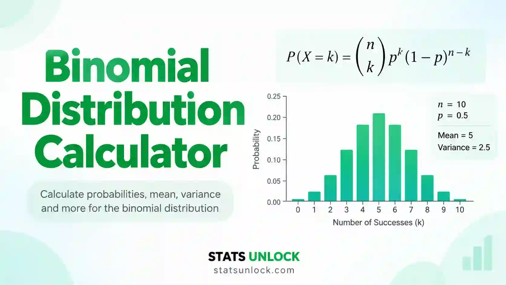

Binomial Distribution Calculator
Find exact binomial probabilities for exactly, at most, at least or between x successes in n trials, with the mean, variance and standard deviation, a full binomial table, and step-by-step working. Paste or upload your own success counts to estimate p, get Clopper-Pearson and Wilson confidence intervals, run the exact binomial test and check the binomial fit.
⚡ 0. Quick Answer
A binomial distribution calculator gives the probability of getting exactly x successes in n independent trials when each trial succeeds with the same probability p.
For example, the chance of exactly 5 heads in 10 fair coin tosses is 0.2461. "At least" and "at most" questions add up the individual probabilities. The mean is np and the standard deviation is √(np(1 − p)).
Rule of thumb: always use the exact binomial value. Use the normal approximation only as a check, and only when both np and n(1 − p) are at least 10.
Key takeaways
- The binomial distribution calculator needs only n (trials), p (chance of success) and x (successes you care about).
- With n = 80 and p = 0.60 the mean is 48 and the standard deviation is 4.38, and P(X ≥ 55) = 0.0675.
- "At least x" is 1 − P(X ≤ x − 1), the step people most often get wrong in Excel, R and Python.
- From real counts, 634 successes in 960 trials gives p̂ = 0.6604 with a 95% exact interval of 0.6295 to 0.6904.
- A dispersion index near 1 means your counts behave like a true binomial; far above 1 means you need a beta-binomial model.
📚 1. What Is the Binomial Distribution?
The binomial distribution describes how many successes you get when you repeat the same yes-or-no trial a fixed number of times. A trial is one attempt: one coin toss, one seed, one patient, one free throw. A success is simply the outcome you are counting. It does not have to be a good thing. A defective item can be a "success" if defects are what you count.
Four conditions make a count binomial. People remember them as BINS:
- B, Binary outcome. Each trial has only two results: success or failure.
- I, Independent trials. One result does not change the chance of the next.
- N, Number of trials is fixed. You decide n before you start.
- S, Same probability. The chance of success p is the same on every trial.
If all four hold, the number of successes X follows a binomial distribution, written X ~ Binomial(n, p) or B(n, p). The distribution tells you the probability of every possible count from 0 to n.
A worked one-liner: a seed supplier says 60% of seeds germinate. You sow 80 seeds in a tray. You expect np = 80 × 0.60 = 48 to germinate, with a standard deviation of √(80 × 0.60 × 0.40) = 4.38. The chance that 55 or more germinate is only 0.0675, so a tray of 55 is unusual but not impossible.
Who uses it: doctors count patients who respond to a drug. Quality engineers count defective items per batch. Ecologists count eggs that hatch per nest. Geneticists count offspring with a trait. Pollsters count yes answers. Sports analysts count made shots. Marketers count visitors who buy. Any time the question is "how many out of n?", the binomial distribution is the starting point.
| Distribution | What it counts | Use it when |
|---|---|---|
| Binomial | Successes in a fixed n trials | n is fixed, p is constant, trials are independent |
| Bernoulli | One trial, 0 or 1 | The binomial with n = 1 |
| Poisson | Events in a time or space with no upper limit | n is huge and p is tiny, or there is no fixed n |
| Hypergeometric | Successes drawn without replacement | Sampling from a small finite population, so p changes each draw |
| Geometric | Trials until the first success | The number of trials is the random part, not the successes |
| Beta-binomial | Successes when p itself varies | Counts vary more than a binomial allows (overdispersion) |
🧮 2. Set Up Your Data
Step A. Describe the binomial experiment
Step B. Add observed success counts (optional)
Each value is the number of successes in one observation of n trials, for example seeds germinated in each tray. Use 0 and 1 with n = 1 for yes-or-no data. Leave the boxes empty if you only need probabilities.
52, 48, 55, 61, 47, .... Spaces, tabs, semicolons and new lines also work. The group name above each box is editable. Nothing is calculated until you press Calculate.Type one count per cell. Each column becomes a group, and the header cells are editable names. Empty cells are ignored.
Step C. Test and interval settings
📊 3. Results
🧠 4. Interpretation of Results, In Detail
4.1 What the headline probability means
The big number at the top of the results is the exact probability for the question you picked. If it says P(X ≥ 55) = 0.0675, it means: if you repeated the whole experiment of 80 trials many times, about 6.75% of those repeats would give 55 or more successes. It is a long-run frequency, not a promise about one run.
Small probabilities do not mean "impossible". A probability of 0.01 still happens once in every hundred repeats. What a small probability does tell you is that, if your values of n and p are correct, the outcome is surprising. When a surprising outcome actually happens, the first thing to doubt is usually the value of p, not your luck.
4.2 Exactly, at most, at least, and between: choosing the right question
Most wrong answers come from asking the wrong question, not from bad arithmetic. Read the words in your problem carefully and match them to the table below.
| Words in the problem | Symbol | How it is computed |
|---|---|---|
| exactly x | P(X = x) | One PMF value |
| at most x, no more than x, x or fewer | P(X ≤ x) | CDF at x |
| fewer than x, less than x | P(X < x) | CDF at x − 1 |
| at least x, x or more, no fewer than x | P(X ≥ x) | 1 − CDF at x − 1 |
| more than x, greater than x | P(X > x) | 1 − CDF at x |
| between a and b, inclusive | P(a ≤ X ≤ b) | CDF at b − CDF at a − 1 |
Because X is a whole number, the difference between "<" and "≤" is a whole bar of the distribution. With continuous distributions such as the normal it makes no difference; with the binomial it can change the answer a lot.
4.3 Mean, variance and standard deviation
The mean μ = np is the number of successes you expect on average. The variance np(1 − p) measures how much the count moves around that average, and the standard deviation is its square root. A handy rule: about 95% of outcomes fall within two standard deviations of the mean when np and n(1 − p) are both reasonably large.
The spread is largest when p = 0.5 and shrinks towards zero as p nears 0 or 1. That is why a 50/50 coin gives much more variable results than a process that almost always succeeds. It is also why the standard error of a proportion is widest at 50%, which is the value survey planners use when they do not know p.
4.4 The mode and the shape
The mode is the single most likely count. It is the whole number part of (n + 1)p. When (n + 1)p is a whole number, there are two modes of equal height, for example n = 9 and p = 0.5 gives modes of 4 and 5.
Skewness tells you which way the tail points. It is zero when p = 0.5, positive when p is below 0.5 (a long tail of large counts) and negative when p is above 0.5. The skew fades as n grows, which is why large binomials look bell-shaped.
4.5 When the normal approximation is safe
Older textbooks approximate the binomial with a normal curve because exact sums were hard to compute by hand. This calculator shows the approximation next to the exact value so you can see the error. The approximation uses a continuity correction: P(X ≥ 55) becomes the normal area above 54.5, because the bar for 55 covers 54.5 to 55.5.
The usual rule is that both np and n(1 − p) should be at least 10, although some books say 5. Even when the rule passes, the approximation is weakest in the tails, which is exactly where p-values live. For reporting, always use the exact value. The approximation is a teaching and checking tool.
4.6 Reading p̂ and its confidence interval
When you enter observed counts, the calculator adds them up and divides by the total number of trials. That pooled proportion is p̂ ("p-hat"), the best single estimate of the true success probability. The confidence interval gives a range of values for the true p that are consistent with your data.
A 95% interval does not mean there is a 95% chance the true p is inside this particular interval. It means that if you repeated the study many times, 95% of the intervals built this way would contain the true p. In practice you can read it as "the plausible range for p". A narrow interval means a precise estimate; it gets narrower roughly with the square root of the number of trials.
4.7 Clopper-Pearson versus Wilson intervals
The Clopper-Pearson interval is called "exact" because it inverts the exact binomial test. It is guaranteed to cover the true p at least 95% of the time, which makes it conservative: it is often a little wider than it needs to be. Regulators and many clinical journals prefer it for exactly that guarantee.
The Wilson score interval is usually a little narrower and has coverage very close to 95% on average. Brown, Cai and DasGupta (2001) recommend it for general use. The simple Wald interval, p̂ ± 1.96·SE, is the one to avoid: it can have coverage far below 95% for small n or for p near 0 or 1, and it can even run below 0. This calculator reports both good intervals so you can choose, and states which one it used.
4.8 The exact binomial test
The exact binomial test asks whether your observed number of successes is consistent with a hypothesised probability p₀. The p-value is the probability, if p₀ were true, of a result at least as extreme as yours. For a two-sided test this calculator uses the same rule as R’s binom.test and SciPy’s binomtest: it adds the probabilities of every count that is no more likely than the one you observed.
A p-value below α (usually 0.05) is called statistically significant. It says the data are hard to explain if p₀ were true. It does not say how big or important the difference is. For that, look at the difference p̂ − p₀, the confidence interval, and Cohen’s h, an effect size for proportions where 0.2 is small, 0.5 medium and 0.8 large.
4.9 The dispersion index and binomial goodness of fit
If your counts are truly binomial, their variance should be close to n·p̂·(1 − p̂). The dispersion index is the observed variance divided by that value. Near 1 means the binomial fits. Clearly above 1 means overdispersion: the counts vary more than a binomial allows, usually because p differs between trays, clinics or litters, or because trials within a group are linked.
The calculator tests this with the chi-square dispersion test described by Tarone (1979). A small p-value for overdispersion is a real warning. The binomial test and intervals will then look more certain than they should, so switch to a beta-binomial or quasi-binomial model. An index well below 1 (underdispersion) is rarer and often means the counts were constrained or recorded with rounding.
Chart 4 shows the same check visually. The bars are how often each count actually occurred; the purple line is how often a binomial with your p̂ says it should occur. Bars that spill wider than the line on both sides are the picture of overdispersion.
4.10 Decision guide
| What you see | What it means | What to do |
|---|---|---|
| Exact test p < α, CI excludes p₀, dispersion OK | Real evidence the rate differs from p₀ | Report p̂, the CI, the p-value and Cohen’s h |
| Exact test p ≥ α, CI includes p₀ | No evidence of a difference | Report the CI width: it shows how large a difference you could have missed |
| Significant, but Cohen’s h < 0.2 | Statistically real but tiny difference, usually from a huge N | Discuss practical importance, not just significance |
| Dispersion index well above 1, test p < 0.05 | Overdispersion, p is not constant | Use beta-binomial or a GLMM with a random effect for group |
| np or n(1 − p) below 10 | Normal approximation unreliable | Use only the exact values, as this calculator does |
| Exact CI and exact test disagree near the edge | Different inversion rules, a known quirk | Report both; the conclusion is borderline |
4.11 Common mistakes this calculator prevents
- Off-by-one in "at least". P(X ≥ x) is 1 − P(X ≤ x − 1), not 1 − P(X ≤ x). The calculator does this for you and shows the step.
- Entering p as a percentage. Typing 60 instead of 0.60 is caught with a clear message.
- Counts larger than n. Any observed value above n or below 0 is flagged, because it cannot come from a binomial.
- Trusting the normal approximation in the tails. The exact value is always the headline; the approximation is shown only as a check with its error.
- Using the Wald interval. It is not reported at all. You get Clopper-Pearson and Wilson.
- Ignoring overdispersion. The fit check runs automatically for every group with two or more observations.
4.12 What the binomial cannot tell you
The binomial model assumes you already know n and that p stays constant. It cannot tell you why the success rate is what it is, and it cannot fix a biased sample: 60 successes from a hand-picked set of 100 trials say nothing reliable about all trials. It also cannot compare two groups formally. For that, use a two-proportion test, Fisher’s exact test or logistic regression, which model the difference directly.
✍ 5. How to Write Your Results in Research
A good binomial result states four things: the count and the total (x out of N), the proportion with a confidence interval, the test and its p-value against a named p₀, and an effect size or plain difference. If you used observed counts, add one sentence on the fit check. Say which interval method you used, because Clopper-Pearson and Wilson give slightly different limits.
📌 Key conventions for this style
- Give the raw count and total, then the percentage: 634 of 960 (66.0%).
- Write p-values without a leading zero: p = .031, and p < .001 for very small values.
- Put the confidence interval in square brackets after the estimate.
- Name the test: "an exact binomial test", not just "a binomial test".
📌 Key conventions for this style
- Justify why the data are binomial: fixed n, two outcomes, independence, constant p.
- Say where p₀ came from: a supplier claim, a historical rate, or chance level.
- Report the fit check and what you would have done if it failed.
- Name the software and interval method.
📌 Key conventions for this style
- Use percentages and "out of", never p̂ or p₀.
- Say "could easily be luck" or "too big to be luck" instead of "significant".
- Give the plausible range as whole percentages.
- Keep it to three short sentences.
📌 Key conventions for this style
- One line per heading, numbers in the Results line only.
- Use three decimal places for proportions.
- Put the key number in bold on a poster.
- Pair the result with Chart 3, which shows p̂, the CI and p₀ together.
📌 Key conventions for this style
- Fix p₀, α, the direction of the test and n before collecting data.
- State the fallback model if overdispersion is found.
- Report the exact software call so others can rerun it.
- Share the raw counts per observation, not just the total.
∑ 6. Formulas Used
🔀 7. Binomial Distribution Calculation Flowchart, Step by Step
This flowchart shows how to calculate a binomial distribution probability step by step, and then how to test real counts against it. Every box uses the same worked example as the Excel, R and Python sections: a supplier claims 60% germination, each tray holds n = 80 seeds, and 12 trays were counted.
Check any box yourself: the Excel sheet in Section 9, the R script in Section 10 and the Python script in Section 11 all return P(X ≥ 55) = 0.0675, p̂ = 0.6604 and an exact p-value of 0.00013 for this dataset.
📝 8. How to Use This Calculator
- Enter the number of trials n. Type n, the fixed number of yes-or-no trials in one experiment, for example 80 seeds per tray.
- Enter the probability of success p. Type p as a decimal from 0 to 1. For 60% type 0.6. If you are testing a claim, this is the hypothesised value p0.
- Pick the probability to find. Choose exactly, at most, fewer than, at least, more than, or between. For between, a second box appears for the upper value.
- Enter x. Type the number of successes you care about, for example 55. The calculator handles the x minus 1 in "at least" for you.
- Add observed counts if you have them. Paste comma-separated success counts such as 52, 48, 55, 61, 47 into a group box. Each value is successes out of n in one observation. Rename the group by typing in its name field.
- Or upload a CSV or Excel file. On the Upload tab choose a file, click every column you want, and press Load. Each selected column becomes its own group.
- Try a sample dataset. Ten built-in datasets cover seeds, clinical trials, free throws, defects, surveys, nests, quizzes, 0/1 conversions, coin tosses and an overdispersed failure case.
- Choose the confidence level and test direction. Pick 90, 95 or 99% and a two-sided or one-sided alternative for the exact binomial test.
- Press Calculate Binomial Probability. Nothing is computed until you press the button, and any change clears old results so you never read stale numbers.
- Read, chart and export. Read the plain-English interpretation, check the four charts and the fit check, copy a reporting template from Section 5, and export a text report or PDF.
📈 9. How to Calculate the Binomial Distribution in Excel
Excel has a full set of binomial functions, so you can calculate any binomial probability without add-ins. The hard parts are knowing which argument makes the result cumulative, getting "at least" right, and building the exact test and confidence interval, which Excel does not provide as single functions. This section walks through all of it with the spreadsheet shown at each stage.
=BINOM.DIST(55,80,0.6,FALSE). Change FALSE to TRUE and you get P(X ≤ 55) instead.9.1 The functions you need
| You want | Excel formula | Note |
|---|---|---|
| P(X = x), binomial pdf | =BINOM.DIST(x,n,p,FALSE) | FALSE means "not cumulative" |
| P(X ≤ x), binomial cdf | =BINOM.DIST(x,n,p,TRUE) | TRUE means cumulative, from 0 up to x |
| P(X ≥ x), at least | =1-BINOM.DIST(x-1,n,p,TRUE) | Note the x − 1 |
| P(a ≤ X ≤ b), between | =BINOM.DIST.RANGE(n,p,a,b) | Excel 2013 and later; inclusive of both ends |
| Smallest x with P(X ≤ x) ≥ α | =BINOM.INV(n,p,alpha) | Replaces the old CRITBINOM |
| n choose x | =COMBIN(n,x) | The binomial coefficient |
| Mean and SD | =n*p and =SQRT(n*p*(1-p)) | No dedicated function |
| Exact 95% CI lower limit | =BETA.INV(0.025,x,N-x+1) | Clopper-Pearson; use 0 if x = 0 |
| Exact 95% CI upper limit | =BETA.INV(0.975,x+1,N-x) | Use 1 if x = N |
BINOMDIST (no dot) still works for old files but is kept only for compatibility, and CRITBINOM has been replaced by BINOM.INV. Use the dotted names so your sheet behaves the same in Excel, Google Sheets and LibreOffice.9.2 Step by step
1 Put n, p and x in their own cells
Never type the numbers straight into the formula. Put n in B1, p in B2 and x in B3 so you can change the question without rewriting anything.
The inputs sit in B1:B3: n = 80 trials, p = 0.60, x = 55.
2 Exactly, at most and at least
Three formulas answer the three most common questions. The "at least" line is where most homework answers go wrong.
=BINOM.DIST(B3,B1,B2,FALSE)=BINOM.DIST(B3,B1,B2,TRUE)=1-BINOM.DIST(B3-1,B1,B2,TRUE)P(X = 55) = 0.0257, P(X ≤ 55) = 0.9583, and P(X ≥ 55) = 0.0675.
3 Mean, variance and standard deviation
=B1*B2=SQRT(B1*B2*(1-B2))These describe the whole distribution, not your particular question, so they stay the same whatever x you choose.
Mean 48, variance 19.2, standard deviation 4.3818.
4 Build a binomial distribution table and graph
Type 0 to 80 down column D. In E2 type =BINOM.DIST(D2,$B$1,$B$2,FALSE) and in F2 =BINOM.DIST(D2,$B$1,$B$2,TRUE), then drag both down. The dollar signs keep n and p fixed as you fill.
=BINOM.DIST(D2,$B$1,$B$2,FALSE)Part of the table around the mean. Column E sums to exactly 1 over all 81 rows, which is a quick check.
5 Estimate p from data, then the exact interval
Put the 12 tray counts in H2:H13. Total successes =SUM(H2:H13) is 634 and total trials =COUNT(H2:H13)*B1 is 960.
=SUM(H2:H13)/(COUNT(H2:H13)*B1)=BETA.INV(0.025,634,960-634+1)=BETA.INV(0.975,634+1,960-634)p̂ = 0.6604, exact 95% CI 0.6295 to 0.6904, the same limits R and Python give.
9.3 The awkward cases: the exact test and the dispersion check
Excel has no BINOM.TEST function. For a one-sided test that the rate is higher than 60%, the p-value is simply P(X ≥ 634) with N = 960:
=1-BINOM.DIST(634-1,960,0.6,TRUE)
That returns 0.000066. For a two-sided test, the quick spreadsheet method doubles the smaller tail:
=MIN(1,2*MIN(BINOM.DIST(634,960,0.6,TRUE),1-BINOM.DIST(633,960,0.6,TRUE)))
This "doubling" rule gives 0.000132, very slightly different from the 0.000130 that R, SciPy and this calculator report, because they add up every outcome that is no more likely than the one observed. With symmetric distributions (p = 0.5) the two rules agree exactly. See 9.4.
The dispersion statistic needs only built-in functions. With p̂ in K1:
=DEVSQ(H2:H13)/(B1*K1*(1-K1))
=CHISQ.DIST.RT(10.79,COUNT(H2:H13)-1)
DEVSQ gives the sum of squared deviations directly. The chi-square is 10.79 on 11 degrees of freedom, p = 0.461, so there is no sign of overdispersion.
9.4 Why your Excel answer might differ from R or Python
| Situation | What happens | Fix |
|---|---|---|
| "At least" gives the wrong answer | You used 1 − BINOM.DIST(x, …, TRUE), which is P(X > x) | Use x − 1 inside the function |
| SciPy "at least" is too small | binom.sf(x) is P(X > x), not P(X ≥ x) | Use binom.sf(x - 1, n, p) |
| Two-sided p-value differs slightly | Excel users often double the tail; R and SciPy use the "minimum likelihood" rule | Report which rule you used; for p₀ = 0.5 they are identical |
| Confidence interval differs | statsmodels proportion_confint defaults to the normal (Wald) method | Pass method="beta" for exact or method="wilson" |
R prop.test disagrees with binom.test | prop.test is a chi-square approximation with continuity correction | Use binom.test for the exact result |
| Tiny probabilities show 0 | Display rounding, not a true zero | Format the cell as Scientific |
| Tool | P(X = x) | P(X ≤ x) | P(X ≥ x) | Exact test |
|---|---|---|---|---|
| Excel / Google Sheets | BINOM.DIST(x,n,p,FALSE) | BINOM.DIST(x,n,p,TRUE) | 1-BINOM.DIST(x-1,n,p,TRUE) | Build by hand |
| R | dbinom(x,n,p) | pbinom(x,n,p) | pbinom(x-1,n,p,lower.tail=FALSE) | binom.test(x,n,p) |
| Python SciPy | binom.pmf(x,n,p) | binom.cdf(x,n,p) | binom.sf(x-1,n,p) | binomtest(x,n,p) |
| TI-84 | binompdf(n,p,x) | binomcdf(n,p,x) | 1-binomcdf(n,p,x-1) | Not built in |
| SPSS | Transform → Compute with PDF.BINOM and CDF.BINOM; Analyze → Nonparametric Tests → Legacy Dialogs → Binomial for the test | |||
9.5 Charting the binomial distribution in Excel
- Select the x column (D) and the P(X = x) column (E) from the table in step 4.
- Insert → Charts → Clustered Column.
- Right-click a bar, choose Format Data Series, and set Gap Width to about 10% so the bars nearly touch, the usual look for a discrete distribution.
- To shade your question region, add a third column with
=IF(D2>=$B$3,E2,0), add it as a second series, and set Series Overlap to 100% with an orange fill. - Label the axes "Number of successes" and "Probability", and put n and p in the title.
Chart 1 in Section 3 of this page draws the same graph with your question shaded automatically.
9.6 Excel errors you will probably hit
| Excel shows | Why | Fix |
|---|---|---|
#NUM! from BINOM.DIST | x > n, x < 0, or p outside 0 to 1 | Check p is a decimal, not a percentage like 60 |
#VALUE! | A cell holds text, for example "80 seeds" | Keep units in a separate label cell |
| Decimals in x are silently cut | Excel truncates 5.7 to 5 without warning | Make sure x and n are whole numbers |
#NAME? | Old Excel (2007 or earlier) has no BINOM.DIST.RANGE | Use two BINOM.DIST calls and subtract |
| At least answer too small | Forgot the x − 1 | =1-BINOM.DIST(x-1,n,p,TRUE) |
BETA.INV returns #NUM! | x = 0 or x = N makes a shape parameter 0 | Set the lower limit to 0 when x = 0 and the upper to 1 when x = N |
| Table does not sum to 1 | Rows stop before n, or $ signs missing so n changed while filling | Fill from 0 to n and lock $B$1, $B$2 |
📈 10. How to Calculate the Binomial Distribution in R
R has the four binomial functions built in: dbinom for the pdf, pbinom for the cdf, qbinom for quantiles and rbinom for random draws, plus binom.test for the exact test. The script below is complete: it answers the probability question, estimates p from the tray counts, runs the exact test, computes both confidence intervals, checks for overdispersion, prints a plain-English verdict and saves one publication-ready figure at 300 dpi. It uses base R only.
Rscript. Change only the four input lines: n, p0, x and counts.10.1 The complete script
R, base only, saves binomial_plot.png
# ============================================================
# Binomial distribution: probabilities, exact test, CI and fit
# StatsUnlock - https://statsunlock.com/binomial-distribution-calculator/
# Base R only. No packages to install.
# ============================================================

# ---- 1. The model and your question ------------------------
n  <- 80       # trials per observation (seeds per tray)
p0 <- 0.60     # claimed probability of success
x  <- 55       # we want P(X >= 55)

# ---- 2. Your observed counts (one value per tray) ----------
# Or read a CSV:
#   counts <- read.csv("data.csv")$germinated
counts <- c(52, 48, 55, 61, 47, 50, 58, 53, 49, 56, 51, 54)
counts <- counts[!is.na(counts)]           # drop missing values

# ---- 3. Probabilities --------------------------------------
cat(sprintf("P(X = %d)  = %.4f\n", x, dbinom(x, n, p0)))
cat(sprintf("P(X <= %d) = %.4f\n", x, pbinom(x, n, p0)))
cat(sprintf("P(X >= %d) = %.4f   # 1 - pbinom(x - 1)\n", x,
            pbinom(x - 1, n, p0, lower.tail = FALSE)))
cat(sprintf("mean = %.4f  variance = %.4f  SD = %.4f\n",
            n * p0, n * p0 * (1 - p0), sqrt(n * p0 * (1 - p0))))

# ---- 4. Estimate p, exact test, confidence intervals -------
k  <- length(counts)
xs <- sum(counts)
N  <- k * n
bt <- binom.test(xs, N, p = p0, alternative = "two.sided", conf.level = 0.95)
ph <- xs / N
z  <- qnorm(0.975)
wil <- (ph + z^2 / (2 * N) + c(-1, 1) * z * sqrt(ph * (1 - ph) / N + z^2 / (4 * N^2))) /
       (1 + z^2 / N)
cat(sprintf("\n%d successes of %d trials, p-hat = %.4f\n", xs, N, ph))
cat(sprintf("95%% CI exact  = [%.4f, %.4f]\n", bt$conf.int[1], bt$conf.int[2]))
cat(sprintf("95%% CI Wilson = [%.4f, %.4f]\n", wil[1], wil[2]))
cat(sprintf("exact binomial test p-value = %.5f\n", bt$p.value))

# ---- 5. Dispersion check (Tarone chi-square) ---------------
D      <- sum((counts - mean(counts))^2) / (n * ph * (1 - ph))
p_disp <- pchisq(D, df = k - 1, lower.tail = FALSE)
cat(sprintf("dispersion chi2(%d) = %.2f, p = %.3f, index = %.2f\n",
            k - 1, D, p_disp, D / (k - 1)))

verdict <- if (bt$p.value < 0.05) "differs from" else "is consistent with"
fit     <- if (p_disp < 0.05) "overdispersed: use a beta-binomial model" else "binomial fit OK"
cat(sprintf("\nVerdict: the germination rate %s %.0f%% (%s).\n", verdict, p0 * 100, fit))

# ---- 6. One 300 dpi figure: PMF with the question shaded ---
set.seed(42)                         # nothing random here, kept for habit
mu <- n * p0; s <- sqrt(n * p0 * (1 - p0))
ks <- max(0, floor(mu - 5 * s)):min(n, ceiling(mu + 5 * s))
png("binomial_plot.png", width = 2700, height = 1650, res = 300)
par(mar = c(5, 5, 5, 2))
bp <- barplot(dbinom(ks, n, p0), names.arg = ks,
              col = ifelse(ks >= x, "#ea580c", "#86efac"), border = "#15803d",
              xlab = "Seeds germinated out of 80", ylab = "Probability", las = 1)
abline(v = bp[ks == round(mu)], col = "#2563eb", lty = 2, lwd = 2)
points(bp[match(counts, ks)], rep(0, k), pch = 17, col = "#7c3aed", cex = 1.4, xpd = TRUE)
title(sprintf("Binomial(n = %d, p = %.2f):  P(X >= %d) = %.4f", n, p0, x,
              pbinom(x - 1, n, p0, lower.tail = FALSE)), adj = 0, line = 2.6)
title(sprintf("purple triangles = observed trays, p-hat = %.3f", ph),
      adj = 0, line = 1.2, font.main = 1, cex.main = 0.9)
legend("topright", bty = "n", fill = c("#ea580c", "#86efac"),
       legend = c(sprintf("X >= %d", x), sprintf("X < %d", x)))
dev.off()
cat("Saved binomial_plot.png\n")
Expected console output: P(X = 55) = 0.0257, P(X ≥ 55) = 0.0675, p-hat = 0.6604, exact CI [0.6295, 0.6904], p-value = 0.00013, dispersion chi2(11) = 10.79, p = 0.461.
10.2 What each part does
| Line or function | What it does, and why it is there |
|---|---|
| dbinom(x, n, p0) | The probability mass function, P(X = x). The "d" stands for density, even though a binomial has probabilities rather than densities. |
| pbinom(x, n, p0) | The cumulative distribution, P(X ≤ x). Always includes x itself. |
| pbinom(x - 1, ..., lower.tail = FALSE) | P(X > x − 1), which is P(X ≥ x). Using lower.tail = FALSE is more accurate than 1 - pbinom() for very small tails. |
| counts[!is.na(counts)] | Removes missing values, because sum() returns NA if any value is missing. |
| binom.test(xs, N, p = p0) | Exact binomial test. Its $p.value uses the minimum-likelihood two-sided rule and $conf.int is the Clopper-Pearson interval. |
| wil <- ... | The Wilson score interval written out from its formula, since base R has no function for it. prop.test(xs, N, correct = FALSE)$conf.int gives the same numbers. |
| D <- sum((counts - mean(counts))^2) / ... | Tarone’s dispersion statistic: the observed spread of the counts divided by the spread a binomial predicts. |
| pchisq(D, df = k - 1, lower.tail = FALSE) | Upper-tail chi-square p-value. Small values mean overdispersion. |
| png(..., res = 300) | Opens a 300 dpi file device. Without res you get a blurry 72 dpi image. |
| barplot(..., col = ifelse(ks >= x, ...)) | Draws the PMF and colours the bars in the question region orange. |
| points(..., pch = 17, xpd = TRUE) | Marks each observed tray as a purple triangle along the axis so data and model sit in one picture. |
| dev.off() | Closes the device and writes the file. Forgetting it leaves an empty PNG. |
10.3 What the figure shows
The bars are the binomial probabilities for every count from about 26 to 70, the range where almost all the probability sits. Bars at 55 and above are orange: their total height is P(X ≥ 55) = 0.0675. The dashed blue line marks the mean, 48. The purple triangles along the bottom are the 12 real trays.
Reading it takes a few seconds. Most triangles sit to the right of the mean, and several are in or near the orange region. That picture already tells you the supplier’s 60% is probably too low, which the exact test then confirms with p = 0.00013.
10.4 Common R problems and fixes
| Symptom | Cause | Fix |
|---|---|---|
| "At least" answer is too small | Used 1 - pbinom(x, n, p) | Use pbinom(x - 1, n, p, lower.tail = FALSE) |
binom.test error "'x' must be nonnegative and integer" | Passed a proportion or a decimal | Pass the count of successes and the number of trials |
| p-value differs from a textbook | The book doubled one tail | Both are valid; state the rule used |
prop.test gives a different CI | It uses a continuity-corrected Wilson interval | Use correct = FALSE for plain Wilson, or binom.test for exact |
dbinom returns 0 with a warning | x was not a whole number | Round or fix the input |
| Empty PNG | dev.off() never ran | Run dev.off() until it reports "null device" |
| Barplot bars and points misaligned | Barplot x positions are not 0, 1, 2 | Use the positions returned by barplot(), as the script does |
10.5 Useful one-liners
| You want | R code |
|---|---|
| Full binomial table | data.frame(x = 0:n, pmf = dbinom(0:n, n, p), cdf = pbinom(0:n, n, p)) |
| Between a and b | sum(dbinom(a:b, n, p)) |
| Quantile, smallest x with P(X ≤ x) ≥ 0.95 | qbinom(0.95, n, p) |
| Simulate 1000 experiments | set.seed(1); rbinom(1000, n, p) |
| One-sided exact test | binom.test(xs, N, p0, alternative = "greater") |
| Many CI methods at once | binom::binom.confint(xs, N) (package binom) |
| Beta-binomial fit if overdispersed | aod::betabin(cbind(x, n - x) ~ 1, ~ 1, data = df) |
| Logistic model with trials | glm(cbind(x, n - x) ~ group, family = binomial, data = df) |
📈 11. How to Calculate the Binomial Distribution in Python
In Python the binomial distribution lives in scipy.stats.binom, and the exact test is scipy.stats.binomtest, which also returns Clopper-Pearson and Wilson intervals. The script below reproduces every number from the R section, prints a plain-English verdict and saves one 300 dpi figure.
n, p0, x and the counts array. Requires SciPy 1.7 or later for binomtest.Install once with pip install numpy scipy matplotlib.
11.1 The complete script
Python 3, saves binomial_plot.png
# ============================================================
# Binomial distribution: probabilities, exact test, CI and fit
# StatsUnlock - https://statsunlock.com/binomial-distribution-calculator/
# Needs: numpy, scipy, matplotlib   (pip install numpy scipy matplotlib)
# ============================================================
import numpy as np
from scipy import stats
import matplotlib
matplotlib.use("Agg")                  # save to file, no window needed
import matplotlib.pyplot as plt

# ---- 1. The model and your question ------------------------
n  = 80        # trials per observation (seeds per tray)
p0 = 0.60      # claimed probability of success
x  = 55        # we want P(X >= 55)

# ---- 2. Your observed counts (one value per tray) ----------
# Or read a CSV:
#   import pandas as pd
#   counts = pd.read_csv("data.csv")["germinated"].dropna().astype(int).to_numpy()
counts = np.array([52, 48, 55, 61, 47, 50, 58, 53, 49, 56, 51, 54])
counts = counts[~np.isnan(counts)].astype(int)   # drop missing values

# ---- 3. Probabilities --------------------------------------
B = stats.binom(n, p0)
print(f"P(X = {x})  = {B.pmf(x):.4f}")
print(f"P(X <= {x}) = {B.cdf(x):.4f}")
print(f"P(X >= {x}) = {B.sf(x - 1):.4f}   # sf(x-1), NOT sf(x)")
print(f"mean = {B.mean():.4f}  variance = {B.var():.4f}  SD = {B.std():.4f}")

# ---- 4. Estimate p, exact test, confidence intervals -------
k, xs = len(counts), int(counts.sum())
N = k * n
res = stats.binomtest(xs, N, p0, alternative="two-sided")
cp = res.proportion_ci(confidence_level=0.95, method="exact")    # Clopper-Pearson
wi = res.proportion_ci(confidence_level=0.95, method="wilson")
print(f"\n{xs} successes of {N} trials, p-hat = {xs / N:.4f}")
print(f"95% CI exact  = [{cp.low:.4f}, {cp.high:.4f}]")
print(f"95% CI Wilson = [{wi.low:.4f}, {wi.high:.4f}]")
print(f"exact binomial test p-value = {res.pvalue:.5f}")

# ---- 5. Dispersion check (Tarone chi-square) ---------------
ph = xs / N
D = ((counts - counts.mean()) ** 2).sum() / (n * ph * (1 - ph))
p_disp = stats.chi2.sf(D, k - 1)
print(f"dispersion chi2({k - 1}) = {D:.2f}, p = {p_disp:.3f}, index = {D / (k - 1):.2f}")

verdict = "differs from" if res.pvalue < 0.05 else "is consistent with"
fit = "overdispersed: use a beta-binomial model" if p_disp < 0.05 else "binomial fit OK"
print(f"\nVerdict: the germination rate {verdict} {p0:.0%} ({fit}).")

# ---- 6. One 300 dpi figure: PMF with the question shaded ---
np.random.seed(42)                     # nothing random here, kept for habit
ks = np.arange(max(0, int(B.mean() - 5 * B.std())), min(n, int(B.mean() + 5 * B.std())) + 1)
fig, ax = plt.subplots(figsize=(9, 5.5))
ax.bar(ks, B.pmf(ks), color=np.where(ks >= x, "#ea580c", "#86efac"),
       edgecolor="#15803d", linewidth=0.6)
ax.axvline(B.mean(), color="#2563eb", ls="--", lw=2, label=f"mean = {B.mean():.0f}")
for c in counts:
    ax.plot(c, -0.002, marker="^", color="#7c3aed", ms=8, clip_on=False)
ax.set_xlabel("Seeds germinated out of 80")
ax.set_ylabel("Probability")
ax.set_title(f"Binomial(n = {n}, p = {p0}):  P(X >= {x}) = {B.sf(x - 1):.4f}\n"
             f"purple triangles = observed trays, p-hat = {ph:.3f}", loc="left")
ax.legend(frameon=False)
fig.tight_layout()
fig.savefig("binomial_plot.png", dpi=300)
print("Saved binomial_plot.png")
Expected output: P(X = 55) = 0.0257, P(X ≥ 55) = 0.0675, p-hat = 0.6604, exact CI [0.6295, 0.6904], Wilson [0.6299, 0.6897], p-value = 0.00013, dispersion chi2(11) = 10.79, p = 0.461.
11.2 What each part does
| Line or function | What it does, and why it is there |
|---|---|
| stats.binom(n, p0) | Creates a "frozen" binomial object so you do not repeat n and p in every call. |
| B.pmf(x), B.cdf(x) | P(X = x) and P(X ≤ x). |
| B.sf(x - 1) | The survival function is P(X > value), so sf(x - 1) gives P(X ≥ x). This is the most common SciPy mistake. |
| stats.binomtest(xs, N, p0) | Exact binomial test, same two-sided rule as R. Returns an object with .pvalue and .proportion_ci(). |
| proportion_ci(method="exact") | Clopper-Pearson interval. method="wilson" gives the Wilson score interval. |
| counts[~np.isnan(counts)] | Drops missing values before summing. |
| stats.chi2.sf(D, k - 1) | Upper-tail p-value for the dispersion statistic. |
| np.where(ks >= x, ...) | Colours the bars in the question region orange. |
| fig.savefig(..., dpi=300) | Writes the print-quality PNG. |
11.3 What the figure shows
It is the same picture as the R figure: binomial probabilities for Binomial(80, 0.6), the P(X ≥ 55) region in orange, the mean as a dashed blue line, and the 12 observed trays as purple triangles below the axis. The title prints P(X ≥ 55) = 0.0675 and p-hat = 0.660.
11.4 Common Python problems and fixes
| Symptom | Cause | Fix |
|---|---|---|
AttributeError: binom_test | binom_test was removed in SciPy 1.12 | Use stats.binomtest(...).pvalue |
| "At least" too small | Used binom.sf(x) | Use binom.sf(x - 1, n, p) |
| CI does not match R | Used statsmodels proportion_confint default | Pass method="beta" (exact) or "wilson" |
ValueError in binomtest | k or n passed as float | Wrap with int() |
| Figure window never appears | The script uses the Agg backend | Open binomial_plot.png, or remove the matplotlib.use line |
| pmf returns nan | p outside 0 to 1 | Divide percentages by 100 |
11.5 Useful one-liners
| You want | Python code |
|---|---|
| Full table | pd.DataFrame({"x": k, "pmf": binom.pmf(k, n, p), "cdf": binom.cdf(k, n, p)}) with k = np.arange(n + 1) |
| Between a and b | binom.cdf(b, n, p) - binom.cdf(a - 1, n, p) |
| Mean, variance, skew, kurtosis | binom.stats(n, p, moments="mvsk") |
| Quantile | binom.ppf(0.95, n, p) |
| Simulate | np.random.default_rng(1).binomial(n, p, size=1000) |
| statsmodels exact CI | proportion_confint(xs, N, method="beta") |
| Normal approximation | norm.sf(x - 0.5, n*p, np.sqrt(n*p*(1-p))) |
📋 12. Reference Tables
12.1 Binomial probability table, P(X = x), n = 10
| x | p = 0.1 | p = 0.2 | p = 0.3 | p = 0.4 | p = 0.5 |
|---|---|---|---|---|---|
| 0 | 0.3487 | 0.1074 | 0.0282 | 0.0060 | 0.0010 |
| 1 | 0.3874 | 0.2684 | 0.1211 | 0.0403 | 0.0098 |
| 2 | 0.1937 | 0.3020 | 0.2335 | 0.1209 | 0.0439 |
| 3 | 0.0574 | 0.2013 | 0.2668 | 0.2150 | 0.1172 |
| 4 | 0.0112 | 0.0881 | 0.2001 | 0.2508 | 0.2051 |
| 5 | 0.0015 | 0.0264 | 0.1029 | 0.2007 | 0.2461 |
| 6 | 0.0001 | 0.0055 | 0.0368 | 0.1115 | 0.2051 |
| 7 | 0.0000 | 0.0008 | 0.0090 | 0.0425 | 0.1172 |
| 8 | 0.0000 | 0.0001 | 0.0014 | 0.0106 | 0.0439 |
| 9 | 0.0000 | 0.0000 | 0.0001 | 0.0016 | 0.0098 |
| 10 | 0.0000 | 0.0000 | 0.0000 | 0.0001 | 0.0010 |
What to conclude: Each column sums to 1. For p above 0.5, read the table with x replaced by n − x and p by 1 − p, because the binomial is symmetric in that way.
12.2 Cumulative binomial table, P(X ≤ x), n = 10
| x | p = 0.1 | p = 0.2 | p = 0.3 | p = 0.4 | p = 0.5 |
|---|---|---|---|---|---|
| 0 | 0.3487 | 0.1074 | 0.0282 | 0.0060 | 0.0010 |
| 1 | 0.7361 | 0.3758 | 0.1493 | 0.0464 | 0.0107 |
| 2 | 0.9298 | 0.6778 | 0.3828 | 0.1673 | 0.0547 |
| 3 | 0.9872 | 0.8791 | 0.6496 | 0.3823 | 0.1719 |
| 4 | 0.9984 | 0.9672 | 0.8497 | 0.6331 | 0.3770 |
| 5 | 0.9999 | 0.9936 | 0.9527 | 0.8338 | 0.6230 |
| 6 | 1.0000 | 0.9991 | 0.9894 | 0.9452 | 0.8281 |
| 7 | 1.0000 | 0.9999 | 0.9984 | 0.9877 | 0.9453 |
| 8 | 1.0000 | 1.0000 | 0.9999 | 0.9983 | 0.9893 |
| 9 | 1.0000 | 1.0000 | 1.0000 | 0.9999 | 0.9990 |
| 10 | 1.0000 | 1.0000 | 1.0000 | 1.0000 | 1.0000 |
What to conclude: For "at least x", take 1 minus the value in the row for x − 1. Example: n = 10, p = 0.5, P(X ≥ 8) = 1 − 0.9453 = 0.0547.
12.3 Mean, SD and the normal-approximation rule
| n | p | Mean np | SD | np / n(1−p) | Normal approx. |
|---|---|---|---|---|---|
| 10 | 0.50 | 5.00 | 1.5811 | 5.00 / 5.00 | Use exact |
| 20 | 0.30 | 6.00 | 2.0494 | 6.00 / 14.00 | Use exact |
| 50 | 0.10 | 5.00 | 2.1213 | 5.00 / 45.00 | Use exact |
| 80 | 0.60 | 48.00 | 4.3818 | 48.00 / 32.00 | Safe |
| 100 | 0.05 | 5.00 | 2.1794 | 5.00 / 95.00 | Use exact |
| 400 | 0.50 | 200.00 | 10.0000 | 200.00 / 200.00 | Safe |
What to conclude: The approximation needs both np and n(1 − p) of at least 10. With p near 0 or 1 you need a much larger n.
12.4 Three 95% confidence interval methods compared
| x / N | p̂ | Wald (avoid) | Wilson | Clopper-Pearson |
|---|---|---|---|---|
| 0 / 20 | 0.000 | [0.000, 0.000] | [0.000, 0.161] | [0.000, 0.168] |
| 2 / 20 | 0.100 | [0.000, 0.231] | [0.028, 0.301] | [0.012, 0.317] |
| 10 / 20 | 0.500 | [0.281, 0.719] | [0.299, 0.701] | [0.272, 0.728] |
| 19 / 20 | 0.950 | [0.854, 1.000] | [0.764, 0.991] | [0.751, 0.999] |
| 5 / 100 | 0.050 | [0.007, 0.093] | [0.022, 0.112] | [0.016, 0.113] |
| 50 / 100 | 0.500 | [0.402, 0.598] | [0.404, 0.596] | [0.398, 0.602] |
What to conclude: With 0 successes the Wald interval collapses to [0, 0], which is plainly wrong. Wilson and Clopper-Pearson stay sensible; Clopper-Pearson is always the widest.
12.5 Cohen’s h effect size bands for proportions
| |h| | Label | Example |
|---|---|---|
| Below 0.20 | Negligible | e.g. 50% vs 55% is h = 0.10 |
| 0.20 to 0.49 | Small | e.g. 50% vs 60% is h = 0.20 |
| 0.50 to 0.79 | Medium | e.g. 50% vs 74% is h = 0.50 |
| 0.80 and above | Large | e.g. 50% vs 88% is h = 0.84 |
What to conclude: Report h beside the p-value. With very large samples even negligible differences become significant.
12.6 Trials needed for "at least one success"
| p per trial | n for P(X ≥ 1) ≥ 0.95 | n for P(X ≥ 1) ≥ 0.99 |
|---|---|---|
| 0.50 | 5 | 7 |
| 0.20 | 14 | 21 |
| 0.10 | 29 | 44 |
| 0.05 | 59 | 90 |
| 0.01 | 299 | 459 |
What to conclude: From P(X ≥ 1) = 1 − (1 − p)n. A 1% event needs 299 trials to be 95% sure of seeing it at least once.
12.7 Total trials for a target 95% margin of error
| Expected p | Margin | Total trials N |
|---|---|---|
| 0.50 | ±10 points | 97 |
| 0.50 | ±5 points | 385 |
| 0.50 | ±3 points | 1068 |
| 0.20 | ±5 points | 246 |
| 0.10 | ±3 points | 385 |
What to conclude: N = 1.96² p(1 − p) ÷ margin². Use p = 0.5 when unsure; it gives the largest N.
📈 13. Example Results
Eight worked examples covering the cases you will actually meet: a textbook problem, a clearly significant result, a borderline one, a null result, a tiny sample, a significant but trivial difference, a failed assumption, and a real applied decision. Every number was computed with the same engine as the calculator.
Heads in 10 fair coin tosses
The classic first binomial problem, done properly.
A fair coin is tossed 10 times. What is the chance of exactly 5 heads, and of 8 or more heads?
| Statistic | Value | Note |
|---|---|---|
| C(10, 5) | 252 | Ways to place 5 heads |
| P(X = 5) | 0.2461 | 252 × 0.5¹⁰ |
| P(X ≤ 7) | 0.9453 | Cumulative |
| P(X ≥ 8) | 0.0547 | 1 − P(X ≤ 7) |
| Mean, SD | 5, 1.5811 | np and √(np(1 − p)) |
What it means: Even for a perfectly fair coin, exactly 5 heads happens only about a quarter of the time. Getting 8 or more heads happens about once in 18 sets of 10 tosses, so it is unusual but not strong evidence the coin is biased.
How to write it: "For a fair coin, P(X = 5) = 0.246 and P(X ≥ 8) = 0.055 in 10 tosses."
Seed germination above the supplier claim
The worked example used in Sections 7, 9, 10 and 11.
Twelve trays of 80 seeds germinated 52, 48, 55, 61, 47, 50, 58, 53, 49, 56, 51 and 54 seeds. The supplier claims 60%.
| Statistic | Value | Note |
|---|---|---|
| p̂ | 0.6604 | 634 ÷ 960 |
| 95% CI exact | [0.6295, 0.6904] | Clopper-Pearson |
| Exact test p | 0.00013 | Two-sided vs 0.60 |
| Cohen's h | 0.125 | Below 0.2, modest |
| Dispersion | index 0.98, p = 0.461 | Binomial fits |
What it means: The true germination rate is very likely between 63% and 69%, above the claimed 60%. The fit check passed, so the p-value is trustworthy. Cohen’s h of 0.13 marks the gain as modest in size, about 6 extra seeds per tray, but consistent across trays.
How to write it: "Germination was 66.0% (634/960), 95% CI [63.0%, 69.0%], higher than the claimed 60%, exact binomial test p < .001, h = 0.12."
Vaccine side-effect rate in a small audit
A p-value just either side of 0.05 needs careful words.
A clinic audits 50 patients. 22 report a mild side effect. The leaflet says 30%.
| Statistic | Value | Note |
|---|---|---|
| p̂ | 0.4400 | 22 ÷ 50 |
| 95% CI exact | [0.2999, 0.5875] | Includes values near 0.30 |
| Exact test p | 0.0433 | Two-sided vs 0.30 |
| Cohen's h | 0.291 | Small to medium |
| P(X ≥ 22 | p = 0.3) | 0.0251 | One tail |
What it means: The exact test gives p = 0.043, just under 0.05, yet the exact 95% interval starts at 0.2999, a hair below 30%. The test and the interval use slightly different rules, and here they land on opposite sides of the line. That is the definition of borderline: the evidence that the true rate exceeds 30% is weak to moderate. The honest conclusion is "possibly higher, collect more data".
How to write it: "22 of 50 patients (44%, 95% CI [30%, 59%]) reported the side effect, compared with 30% expected, exact binomial test p = .043."
Village survey support near 50%
No difference is a result too, if the interval is reported.
A survey of 200 residents finds 108 in favour of a new market. Is support different from 50%?
| Statistic | Value | Note |
|---|---|---|
| p̂ | 0.5400 | 108 ÷ 200 |
| 95% CI exact | [0.4683, 0.6105] | Contains 0.50 |
| Exact test p | 0.2888 | Two-sided vs 0.50 |
| Cohen's h | 0.080 | Negligible |
| Mean under H₀ | 100 | np |
What it means: There is no evidence that support differs from 50%. The interval shows support could plausibly be anywhere from about 47% to 61%, so the survey cannot rule out a modest majority either way.
How to write it: "108 of 200 residents (54%, 95% CI [47%, 61%]) supported the market, not significantly different from 50%, exact binomial test p = .29."
Seven of eight nests hatched
Where the normal approximation fails and only the exact test is honest.
A field team finds 8 nests; 7 hatched at least one egg. Is the hatch rate above 50%?
| Statistic | Value | Note |
|---|---|---|
| Exact test p | 0.0703 | Two-sided vs 0.50 |
| Normal approx. z-test p | 0.0339 | Without correction, misleading |
| 95% CI exact | [0.4735, 0.9968] | Very wide |
| np, n(1 − p) | 4, 4 | Fails the rule of 10 |
| P(X ≥ 7) | 0.0352 | One tail |
What it means: A naive z-test would call this significant (p ≈ 0.03), but the exact test gives p = 0.07. With only 8 nests the interval runs from about 47% to nearly 100%. Report the exact result and say the sample is too small to be sure.
How to write it: "Seven of eight nests hatched (87.5%, 95% CI [47.3%, 99.7%]), exact binomial test p = .070."
A very large A/B click test
A huge N makes a tiny difference significant.
A website shows a button 100,000 times and records 50,500 clicks on the new colour versus 50% expected.
| Statistic | Value | Note |
|---|---|---|
| p̂ | 0.5050 | 50,500 ÷ 100,000 |
| 95% CI exact | [0.5019, 0.5081] | Very narrow |
| Exact test p | 0.0016 | Significant |
| Cohen's h | 0.0100 | Far below 0.2 |
| Difference | +0.5 points | Practically tiny |
What it means: The difference is real in the statistical sense but only half a percentage point. Whether that matters is a business question, not a statistical one. Always show the effect size beside the p-value.
How to write it: "The click rate was 50.5% (95% CI [50.2%, 50.8%]), p = .002, but the effect was negligible (h = 0.01)."
Mixed seed lots, strong overdispersion
The binomial looks fine on paper and fails in the data.
Twelve trays of 20 seeds from different lots germinated 2, 18, 5, 19, 3, 17, 1, 20, 4, 16, 6 and 18 seeds.
| Statistic | Value | Note |
|---|---|---|
| p̂ | 0.5375 | Close to 0.5 |
| Observed variance | 59.84 | Of the tray counts |
| Binomial variance | 4.97 | n p̂ (1 − p̂) |
| Dispersion χ²(11) | 132.4, p = 5.7e-23 | Overdispersed |
| Exact test vs 0.5 | 0.2725 | Not trustworthy here |
What it means: The pooled rate is near 50%, but no tray is near 50%: some lots germinate almost fully and others almost not at all. The dispersion index of about 12 shows the binomial model is wrong. Analyse lots separately or fit a beta-binomial.
How to write it: "Tray counts were strongly overdispersed (χ²(11) = 132.4, p < .001), so a beta-binomial model was used instead of the binomial."
Quality control alarm rule
Using "at least" probabilities to set an action limit.
A line has a 4% defect target. Each batch has 50 items. How rare is a batch with 5 or more defects if the line is on target?
| Statistic | Value | Note |
|---|---|---|
| P(X = 0) | 0.1299 | Defect-free batch |
| P(X ≤ 2) | 0.6767 | At or below the mean |
| P(X ≥ 5) | 0.0490 | False-alarm rate |
| P(X ≥ 6) | 0.0144 | Stricter limit |
| Poisson approx. P(X ≥ 5) | 0.0527 | λ = 2 |
What it means: If the line is on target, only about 5% of batches would show 5 or more defects, so 5 is a sensible alarm point with a 1-in-20 false-alarm rate. Using 6 lowers false alarms to about 1.4% but reacts more slowly.
How to write it: "With p = 0.04 and 50 items per batch, P(X ≥ 5) = 0.049, so batches with five or more defects trigger inspection."
🧪 14. Data Collection Protocol
Study design: the binomial model assumes repeated observations of a fixed number of independent yes-or-no trials, each with the same probability of success. Collect data so that every one of those conditions is true by design, not by hope.
- Define "success" in writing before you start. A germinated seed must mean something exact, for example a radicle at least 2 mm long after 7 days. Vague definitions let the rate drift between observers.
- Fix n for every observation. Sow exactly 80 seeds per tray, give exactly 20 patients per clinic the treatment, take exactly 10 shots per session. If n must vary, record it per row and analyse proportions with a binomial GLM instead.
- Make trials independent. Randomise the order, keep physical separation where contagion or crowding could link outcomes, and avoid scoring the same subject twice.
- Keep p constant within a group. Use one seed lot, one supplier, one protocol. If you suspect p differs between sites or days, make those separate groups so the calculator tests each one.
- Decide p₀ and where it comes from. A supplier claim, a historical rate, a regulatory limit, or chance level (0.5 for a coin, 0.25 for four-option guessing). Write it down with its source.
- Choose one-sided or two-sided before seeing data. One-sided is only honest when a result in the other direction would lead to the same action as no result.
- Plan the total number of trials. The width of a 95% interval is about 2 × 1.96 × √[p(1 − p) ÷ N]. For ±5 percentage points at p = 0.5 you need about 385 trials in total.
- Record counts, not percentages. Store "52 of 80", never "65%". Percentages lose n and cannot be tested.
- Record missing observations as blank, never as 0. A zero is a real outcome (no successes); a blank is no data.
- Lay the data out one column per group, one row per observation, exactly as below, ready to paste or upload.
| Tray batch A (germinated of 80) | Tray batch B (germinated of 80) | Tray batch C (germinated of 80) |
|---|---|---|
| 52 | 49 | 55 |
| 48 | 51 | 57 |
| 55 | 47 | 53 |
One column per group, whole-number counts only below the header row. Blank cells are ignored, so unequal numbers of observations per group are fine. Every value must lie between 0 and n.
Minimum sample: the exact test works for any N, but power is low when N is small. For the dispersion check you need at least 2 observations per group, and 8 or more to detect moderate overdispersion.
Pre-registration: record n, p₀, the test direction, α, the interval method (Clopper-Pearson or Wilson) and the fallback model for overdispersion before collecting data.
Common collection mistakes:
- Letting n change silently between observations, for example trays with 78 or 83 seeds.
- Scoring successes from the same litter, class or plot as if they were independent.
- Mixing seed lots or clinics with different true rates into one group.
- Recording percentages or rounding counts, which destroys the binomial structure.
- Choosing p₀ or a one-sided test after looking at the result.
🎯 15. When to Use This Calculator
Use a binomial distribution calculator whenever the question is "how many successes out of a fixed number of tries?"
Use it when:
- ✓ Each trial has exactly two outcomes.
- ✓ The number of trials n is fixed in advance.
- ✓ Trials are independent of each other.
- ✓ The probability of success is the same on every trial.
- ✓ You want an exact probability, a test against a known rate, or a confidence interval for one proportion.
Do not use it when:
- ✗ You sample without replacement from a small population (more than about 5% of it). Use the hypergeometric distribution.
- ✗ There is no fixed n, only a rate of events in time or space. Use the Poisson distribution.
- ✗ You count trials until the first success. Use the geometric distribution.
- ✗ There are three or more outcomes. Use the multinomial distribution.
- ✗ p varies between groups and you want to model why. Use logistic regression or a beta-binomial model.
- ✗ You compare two proportions. Use a two-proportion z-test or Fisher’s exact test.
Real-world examples:
- Agriculture: is a seed lot’s germination rate really 60%?
- Medicine: does a new drug beat the historical 40% response rate?
- Manufacturing: is a batch with 5 defects out of 50 evidence the line is above its 4% target?
- Genetics: do offspring follow a 3:1 Mendelian ratio (p = 0.75)?
- Education: is a student scoring 10 of 20 on a four-option quiz above chance?
- Ecology: what share of nests hatch all four eggs?
- Marketing: what conversion rate is plausible after 400 visits with 38 sales?
Design guidance: plan the number of trials from the interval width you need, keep n identical across observations, and randomise the order of trials.
Decision tree: two outcomes and fixed n? → binomial. No fixed n, just a rate? → Poisson. Drawing without replacement from a small pool? → hypergeometric. Counts vary far more than binomial? → beta-binomial. Comparing two groups? → Fisher’s exact or two-proportion test. Explaining p with predictors? → logistic regression.
🔧 16. Troubleshooting and Common Errors
My "at least" answer is too small
Cause: You computed 1 − P(X ≤ x), which is P(X > x).
Fix: Use 1 − P(X ≤ x − 1). Choose "at least" in the calculator and it does this for you.
I get an error that p must be between 0 and 1
Cause: p was typed as a percentage, for example 60.
Fix: Type 0.60. Divide any percentage by 100.
A group is rejected with "every value must be from 0 to n"
Cause: A count is larger than n, negative, or a decimal, or n is set wrongly.
Fix: Check n matches the trials per observation, and fix typos such as 552 for 55.
The dispersion check shows "Overdispersed"
Cause: p differs between observations or trials are clustered.
Fix: Split the data into more homogeneous groups, or fit a beta-binomial or binomial GLMM in R or Python.
My p-value differs slightly from my textbook or Excel
Cause: Different two-sided rules: doubling the smaller tail versus the minimum-likelihood rule.
Fix: Both are accepted. This calculator matches R binom.test and SciPy binomtest. State which rule you used.
My confidence interval differs from statsmodels
Cause: statsmodels proportion_confint defaults to the Wald (normal) method.
Fix: Pass method="beta" for Clopper-Pearson or method="wilson".
The CI and the test disagree about significance
Cause: The Clopper-Pearson interval and the minimum-likelihood test invert slightly different rules.
Fix: This only happens right at the edge. Report both and describe the result as borderline.
The normal approximation is far from the exact value
Cause: np or n(1 − p) is below 10, or you are in the far tail.
Fix: Use the exact value. The approximation is shown only for comparison.
Charts 3 and 4 are faded
Cause: No observed counts were entered.
Fix: Paste counts into a group, upload a file, or load a sample dataset, then press Calculate.
Uploaded columns do not appear as buttons
Cause: Only columns that are at least 80% numeric are offered, and row 1 must be a header.
Fix: Remove text notes from the data rows and put column names in row 1.
The results disappeared after I edited a value
Cause: Any change clears old results on purpose so you never read stale numbers.
Fix: Press Calculate again.
⚖ 17. Assumptions and Limitations
Assumptions
- Binary outcomes. Check: every trial is scored success or failure. If it fails: forcing three outcomes into two throws information away; use the multinomial.
- Fixed number of trials. Check: n is the same for every observation. If it fails: pooled p̂ is biased towards observations with more trials; use a binomial GLM with trials as weights.
- Independent trials. Check: the design, and the dispersion index. If it fails: positive dependence inflates variance, so p-values are too small and intervals too narrow (anti-conservative).
- Constant probability p. Check: the Tarone dispersion test and Chart 4. If it fails: overdispersion, with the same anti-conservative bias; use beta-binomial or a GLMM.
- Correct p₀. Check: its source. If it fails: every probability and test is answered for the wrong model.
- Representative sampling. Check: how observations were chosen. If it fails: p̂ is precisely wrong, biased in the direction of the selection.
Limitations
- The Clopper-Pearson interval is conservative: its coverage is above the nominal level, so it is wider than necessary. The Wilson interval is shown for a tighter alternative.
- The exact test is discrete, so its true type I error rate is at or below α, never exactly α. A mid-p value is a common, less conservative alternative.
- The dispersion test has low power with few observations; passing it with k = 3 proves little.
- The normal approximation is shown only as a check and can be badly wrong in the tails or when np < 10.
- The calculator tests one group at a time against p₀. It does not compare groups with each other; use Fisher’s exact test or logistic regression.
- It does not fit a beta-binomial model. When overdispersion is flagged, refit in R (
aod,VGAM) or Python (statsmodels). - n is limited to 100,000 per observation for speed in the browser. Beyond that, the normal approximation is extremely accurate anyway.
🏁 18. Conclusion
A binomial distribution calculator answers one of the most common questions in statistics: how likely is a given number of successes when you repeat the same yes-or-no trial a fixed number of times? Three inputs, n, p and x, are enough to give the exact probability for exactly, at most, at least or between, together with the mean np, the variance np(1 − p) and the standard deviation.
The arithmetic is not the hard part. The hard parts are asking the right question and checking the model. "At least 55" is 1 − P(X ≤ 54), not 1 − P(X ≤ 55), and that single off-by-one error causes more wrong homework answers and wrong Excel sheets than anything else in this topic. Always read the words of the problem and match them to the correct symbol before you calculate.
When you have real data, the binomial becomes a tool for inference. Pool the counts to estimate p̂, give it an exact Clopper-Pearson or Wilson confidence interval, and use the exact binomial test to compare it with a claimed rate. Report the count and total, the interval, the p-value and an effect size, so readers can judge both significance and importance. In the worked example, 634 germinations out of 960 seeds gave p̂ = 0.660, well above the claimed 60%, with p = 0.00013.
Finally, never skip the fit check. The binomial assumes one constant p and independent trials. If your counts vary much more than a binomial allows, the dispersion index will rise well above 1 and every p-value will look more convincing than it should. That is the signal to move to a beta-binomial or mixed model rather than to report a false certainty.
Enter your n, p and x above, add your counts if you have them, and read the plain-English interpretation before you write anything down. Then use the five reporting templates to put the result into your paper, thesis or report. Come back to this binomial distribution calculator whenever you need an exact binomial probability, a binomial test or a confidence interval for a proportion.
❓ 19. Frequently Asked Questions
Q1. What is a binomial distribution calculator?
A binomial distribution calculator finds the probability of getting a certain number of successes in a fixed number of independent trials, when every trial has the same chance of success. You enter n, p and x, and it returns P(X = x), P(X ≤ x), P(X ≥ x) or a range, plus the mean, variance and standard deviation.
Q2. What is the binomial probability formula?
P(X = x) = C(n, x) · p^x · (1 − p)^(n − x), where C(n, x) = n! / [x!(n − x)!] counts the ways x successes can be arranged among n trials. For n = 10, p = 0.5 and x = 5 this gives 252 × 0.5^10 = 0.2461.
Q3. How do you calculate a binomial distribution step by step?
First check the four conditions: two outcomes, fixed n, independent trials and constant p. Then write down n, p and x, compute C(n, x), multiply by p^x and (1 − p)^(n − x), and for cumulative questions add the individual probabilities. The step-by-step box in the results shows every stage with your numbers.
Q4. How do I find "at least" binomial probability?
Use the complement: P(X ≥ x) = 1 − P(X ≤ x − 1). For n = 80, p = 0.6 and at least 55 successes, P(X ≤ 54) = 0.9325, so P(X ≥ 55) = 0.0675. The most common mistake is subtracting P(X ≤ x) instead of P(X ≤ x − 1).
Q5. What is the difference between binomial pdf and binomial cdf?
The binomial pdf (more correctly the PMF) gives the probability of exactly x successes. The binomial cdf gives the probability of x or fewer successes, which is the sum of the PMF from 0 to x. On a TI-84 these are binompdf and binomcdf.
Q6. How do you find the mean and standard deviation of a binomial distribution?
The mean is μ = np and the standard deviation is σ = √[np(1 − p)]. For n = 80 and p = 0.6 the mean is 48 and the standard deviation is √19.2 = 4.38. The variance is np(1 − p) = 19.2.
Q7. How do I calculate the binomial distribution in Excel?
Use =BINOM.DIST(x, n, p, FALSE) for exactly x and =BINOM.DIST(x, n, p, TRUE) for x or fewer. For at least x use =1-BINOM.DIST(x-1, n, p, TRUE), and for a range use =BINOM.DIST.RANGE(n, p, a, b). Excel has no exact binomial test function, so build the p-value from BINOM.DIST.
Q8. How do I calculate the binomial distribution in R?
Use dbinom(x, n, p) for P(X = x), pbinom(x, n, p) for P(X ≤ x) and pbinom(x - 1, n, p, lower.tail = FALSE) for P(X ≥ x). For the exact test use binom.test(successes, trials, p = p0), which also returns the Clopper-Pearson confidence interval.
Q9. How do I calculate the binomial distribution in Python with SciPy?
Use scipy.stats.binom.pmf(x, n, p), binom.cdf(x, n, p) and binom.sf(x - 1, n, p) for at least x. For the exact test use scipy.stats.binomtest(k, n, p0); its proportion_ci(method="exact") gives the Clopper-Pearson interval and method="wilson" the Wilson interval. The old binom_test function was removed in SciPy 1.12.
Q10. When can I use the normal approximation to the binomial?
When both np and n(1 − p) are at least 10 (some books say 5). Use a continuity correction: P(X ≥ 55) becomes the normal area above 54.5. Even then it is least accurate in the tails, so report the exact binomial value, which this calculator always gives.
Q11. What is an exact binomial test?
It tests whether an observed number of successes is consistent with a hypothesised probability p0, using the binomial distribution directly rather than an approximation. The two-sided p-value adds the probabilities of all outcomes no more likely than the observed one, the same rule used by R binom.test and SciPy binomtest.
Q12. Which confidence interval should I use for a binomial proportion?
Use the Wilson score interval for general reporting, or the Clopper-Pearson exact interval when you need guaranteed coverage, for example in clinical or regulatory work. Avoid the simple Wald interval p̂ ± 1.96·SE, which can have poor coverage for small samples or extreme p.
Q13. What are the four conditions of a binomial experiment?
Binary outcomes, Independent trials, a fixed Number of trials, and the Same probability of success on every trial, often remembered as BINS. If any one fails, a different distribution such as the hypergeometric, Poisson or beta-binomial may fit better.
Q14. What is overdispersion in binomial data?
Overdispersion means the counts vary more than a binomial with a single p allows, usually because p differs between groups or trials are clustered. The dispersion index is then well above 1. It makes binomial p-values too small, so use a beta-binomial or quasi-binomial model instead.
Q15. How do I test binomial goodness of fit?
Compare the observed variance of your counts with the binomial variance n·p̂(1 − p̂). The Tarone chi-square dispersion statistic D = Σ(xᵢ − x̄)² / [n p̂(1 − p̂)] follows a chi-square distribution with k − 1 degrees of freedom. This calculator runs it automatically and shows observed against expected counts in Chart 4.
Q16. What is the probability of x successes in n trials?
It is P(X = x) = C(n, x) · p^x · (1 − p)^(n − x). For example, the probability of exactly 6 successes in 20 trials with p = 0.3 is 0.1916, and the probability of 6 or fewer is 0.6080.
Q17. How do I calculate binomial probability between two values?
Add the probabilities from the lower to the upper value inclusive: P(a ≤ X ≤ b) = P(X ≤ b) − P(X ≤ a − 1). Choose the "between two values" option in the calculator, or use BINOM.DIST.RANGE(n, p, a, b) in Excel.
Q18. What is the difference between binomial and Poisson distributions?
The binomial counts successes out of a fixed number of trials, so it can never exceed n. The Poisson counts events with no upper limit, such as calls per hour. When n is large and p is small, the Poisson with λ = np closely approximates the binomial.
Q19. What is the difference between binomial and beta-binomial?
The binomial assumes one fixed p. The beta-binomial lets p vary from observation to observation according to a beta distribution, which adds extra variance. Use it when your binomial data are overdispersed, for example litters, clinics or seed lots that differ in their true success rate.
Q20. Can I use this binomial calculator for my thesis or published research?
Yes for exploration, teaching and checking hand calculations. The calculator uses exact formulas that match R and SciPy to four or more decimal places. For formal work, state the model, the test and interval methods, and reproduce the result with the R or Python script in Sections 10 and 11 so your analysis is fully reproducible.
📑 20. Cite This Tool
StatsUnlock. (2026). Binomial distribution calculator [Interactive statistical tool]. https://statsunlock.com/binomial-distribution-calculator/@misc{statsunlock_binomial_2026, title={Binomial Distribution Calculator}, author={{StatsUnlock}}, year={2026}, note={Interactive statistical tool}, url={https://statsunlock.com/binomial-distribution-calculator/}}Binomial probabilities were computed with the StatsUnlock Binomial Distribution Calculator (2026) using exact binomial formulas, with n = ___ and p = ___. Run the calculator to fill in your numbers.🔗 21. Related Tools
The bell curve behind the normal approximation to the binomial.
For counts with no fixed n, or when n is large and p is tiny.
The single-trial case of the binomial, with n = 1.
The large-sample alternative to the exact binomial test.
Compare the success rates of two groups.
Compare two binomial proportions exactly with a 2 × 2 table.
Test observed counts against any expected distribution.
Intervals and tests for one proportion from a count and a total.
90, 95 and 99% intervals for means and proportions.
Model how a binomial success rate changes with predictors.
📖 22. Glossary of Terms
| Term | Plain-English meaning |
|---|---|
| Bernoulli trial | A single trial with two outcomes, success or failure. |
| Beta-binomial distribution | A version of the binomial where p itself varies, used when counts are more spread out than a binomial allows. |
| Binomial coefficient | C(n, x), the number of ways to choose which x of the n trials are successes. |
| Binomial distribution | The distribution of the number of successes in n independent trials with the same probability p. |
| CDF (cumulative distribution function) | The probability of x or fewer successes, P(X ≤ x). |
| Clopper-Pearson interval | An "exact" confidence interval for a proportion built from the binomial distribution; guaranteed coverage but slightly wide. |
| Cohen’s h | An effect size for the difference between two proportions, using an arcsine scale. 0.2 is small, 0.5 medium, 0.8 large. |
| Complement rule | P(event) = 1 − P(not event). Used for "at least" questions. |
| Confidence interval | A range of plausible values for the true proportion, built so that a stated share of such ranges contain it. |
| Continuity correction | Adding or subtracting 0.5 when a normal curve approximates whole-number counts. |
| Dispersion index | Observed variance divided by binomial variance. About 1 fits the binomial; above 1 is overdispersion. |
| Exact binomial test | A hypothesis test for one proportion that uses binomial probabilities directly, with no approximation. |
| Independence | The result of one trial does not change the probability of another. |
| Mean (expected value) | The average number of successes over many repeats, np. |
| Mode | The most likely number of successes, the whole-number part of (n + 1)p. |
| Normal approximation | Using a normal curve with mean np and SD √[np(1 − p)] in place of the binomial when n is large. |
| Overdispersion | More variation in counts than the binomial predicts, usually from varying p or clustered trials. |
| p̂ (p-hat) | The observed proportion of successes, total successes divided by total trials. |
| p-value | The probability, if the null hypothesis were true, of a result at least as extreme as the one observed. |
| PMF (probability mass function) | The probability of exactly x successes, P(X = x). Often called the binomial pdf. |
| Standard deviation | The typical distance of the count from its mean, √[np(1 − p)]. |
| Survival function | The probability of more than a value, P(X > x). In SciPy, sf(x − 1) gives P(X ≥ x). |
| Variance | The average squared distance from the mean, np(1 − p). |
| Wilson score interval | A confidence interval for a proportion with coverage close to the stated level; recommended for general use. |
📚 23. References
These peer-reviewed articles support the methods used in this binomial distribution calculator: exact and approximate confidence intervals, the exact binomial test, the normal approximation, overdispersion and the software used in the worked examples.
- Agresti, A., & Caffo, B. (2000). Simple and effective confidence intervals for proportions and differences of proportions result from adding two successes and two failures. The American Statistician, 54(4), 280–288. https://doi.org/10.1080/00031305.2000.10474560
- Agresti, A., & Coull, B. A. (1998). Approximate is better than “exact” for interval estimation of binomial proportions. The American Statistician, 52(2), 119–126. https://doi.org/10.1080/00031305.1998.10480550
- Blyth, C. R. (1986). Approximate binomial confidence limits. Journal of the American Statistical Association, 81(395), 843–855. https://doi.org/10.1080/01621459.1986.10478343
- Brown, L. D., Cai, T. T., & DasGupta, A. (2001). Interval estimation for a binomial proportion. Statistical Science, 16(2), 101–133. https://doi.org/10.1214/ss/1009213286
- Clopper, C. J., & Pearson, E. S. (1934). The use of confidence or fiducial limits illustrated in the case of the binomial. Biometrika, 26(4), 404–413. https://doi.org/10.1093/biomet/26.4.404
- Fagerland, M. W., Lydersen, S., & Laake, P. (2015). Recommended confidence intervals for two independent binomial proportions. Statistical Methods in Medical Research, 24(2), 224–254. https://doi.org/10.1177/0962280211415469
- Greenland, S., Senn, S. J., Rothman, K. J., Carlin, J. B., Poole, C., Goodman, S. N., & Altman, D. G. (2016). Statistical tests, P values, confidence intervals, and power: A guide to misinterpretations. European Journal of Epidemiology, 31(4), 337–350. https://doi.org/10.1007/s10654-016-0149-3
- Hinde, J., & Demétrio, C. G. B. (1998). Overdispersion: Models and estimation. Computational Statistics & Data Analysis, 27(2), 151–170. https://doi.org/10.1016/S0167-9473(98)00007-3
- Newcombe, R. G. (1998). Two-sided confidence intervals for the single proportion: Comparison of seven methods. Statistics in Medicine, 17(8), 857–872. https://doi.org/10.1002/(SICI)1097-0258(19980430)17:8<857::AID-SIM777>3.0.CO;2-E
- Schader, M., & Schmid, F. (1989). Two rules of thumb for the approximation of the binomial distribution by the normal distribution. The American Statistician, 43(1), 23–24. https://doi.org/10.1080/00031305.1989.10475601
- Skellam, J. G. (1948). A probability distribution derived from the binomial distribution by regarding the probability of success as variable between the sets of trials. Journal of the Royal Statistical Society: Series B, 10(2), 257–261. https://doi.org/10.1111/j.2517-6161.1948.tb00014.x
- Tarone, R. E. (1979). Testing the goodness of fit of the binomial distribution. Biometrika, 66(3), 585–590. https://doi.org/10.1093/biomet/66.3.585
- Thulin, M. (2014). The cost of using exact confidence intervals for a binomial proportion. Electronic Journal of Statistics, 8(1), 817–840. https://doi.org/10.1214/14-EJS909
- Virtanen, P., Gommers, R., Oliphant, T. E., et al. (2020). SciPy 1.0: Fundamental algorithms for scientific computing in Python. Nature Methods, 17, 261–272. https://doi.org/10.1038/s41592-019-0686-2
- Vollset, S. E. (1993). Confidence intervals for a binomial proportion. Statistics in Medicine, 12(9), 809–824. https://doi.org/10.1002/sim.4780120902
- Wallis, S. (2013). Binomial confidence intervals and contingency tests: Mathematical fundamentals and the evaluation of alternative methods. Journal of Quantitative Linguistics, 20(3), 178–208. https://doi.org/10.1080/09296174.2013.799918
- Warton, D. I., & Hui, F. K. C. (2011). The arcsine is asinine: The analysis of proportions in ecology. Ecology, 92(1), 3–10. https://doi.org/10.1890/10-0340.1
- Wasserstein, R. L., & Lazar, N. A. (2016). The ASA statement on p-values: Context, process, and purpose. The American Statistician, 70(2), 129–133. https://doi.org/10.1080/00031305.2016.1154108
- Williams, D. A. (1982). Extra-binomial variation in logistic linear models. Journal of the Royal Statistical Society: Series C (Applied Statistics), 31(2), 144–148. https://doi.org/10.2307/2347977
- Wilson, E. B. (1927). Probable inference, the law of succession, and statistical inference. Journal of the American Statistical Association, 22(158), 209–212. https://doi.org/10.1080/01621459.1927.10502953