

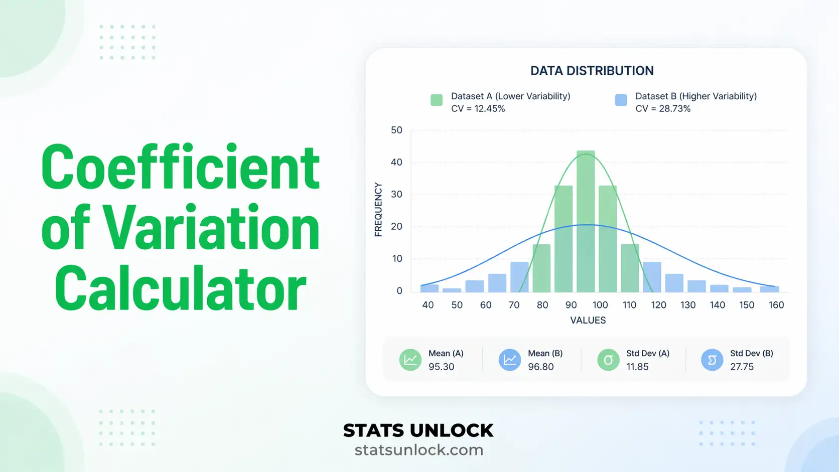

Coefficient of Variation Calculator
Paste comma-separated numbers or upload a CSV and get the coefficient of variation as a percentage, together with the mean, standard deviation, relative standard deviation, a confidence interval and an interpretation band, for one group or several compared side by side.
⚡ 0. Quick Answer
The coefficient of variation (CV) is the standard deviation divided by the mean, expressed as a percentage. It measures how big the spread is relative to the size of the thing being measured.
Because it has no units, the CV lets you compare variability between quantities measured on completely different scales, such as the consistency of a balance weighing in grams against a pipette dispensing in microlitres. A standard deviation of 5 means very different things on a mean of 10 and a mean of 1000; the CV tells them apart.
Rule of thumb: under 10% is low variability, 10 to 20% is moderate, 20 to 30% is high, and above 30% the data are very variable. Laboratory assays usually demand a CV under 15%.
Key takeaways
- CV = (SD / mean) × 100, a unit-free percentage that expresses spread relative to the average.
- The relative standard deviation (RSD) is the same number. Analytical chemistry says RSD, statistics says CV, and both mean SD divided by the mean.
- The CV only works on a ratio scale with a true zero. It is meaningless for Celsius temperature, calendar years, pH, or any scale where zero is arbitrary.
- The most common error is using it when the mean is close to zero, where the CV explodes toward infinity and tells you nothing.
- A lower CV means more consistent measurements, which is why labs, manufacturing and finance all use it as a precision or risk-per-unit-return score.
📚 1. What Is the Coefficient of Variation?
The coefficient of variation answers a question the standard deviation cannot: is this spread large or small for numbers of this size? A standard deviation of 3 kg is enormous if you are weighing mice and trivial if you are weighing cattle. Dividing the standard deviation by the mean cancels the units, leaving a pure ratio that you can multiply by 100 and read as a percentage. That is the entire idea, and it is why the CV appears under different names in almost every applied field.
What this calculator reports for each group:
- CV (%), the coefficient of variation as a percentage, the headline number.
- CV (ratio), the same value before multiplying by 100, which some software reports instead.
- Mean and standard deviation, in your original units, so you can see what the CV was built from.
- Interpretation band, low, moderate, high or very high, based on the conventional thresholds.
- Confidence interval for the CV, an approximate range for the true population value.
- Signal-to-noise ratio, the inverse of the CV, used in engineering and imaging.
- Validity checks, flagging negative values, a mean near zero, or mixed signs, all of which make the CV unusable.
A worked one-liner: if a set of leaf measurements averages 52.44 mm with a standard deviation of 4.19 mm, the coefficient of variation is 4.19 / 52.44 = 0.08, or 8.0%, which counts as low variability.
Who uses it, and what they call it: analytical chemists and clinical laboratories call it the relative standard deviation and use it as the core precision metric for an assay. Haematologists meet it as red cell distribution width, which is literally the CV of red blood cell volume. Cardiologists compute the CV of RR intervals as a heart-rate-variability index. Finance uses it as risk per unit of return, where a lower CV means a better risk-adjusted investment. Biologists use it to compare morphological variability across species of very different body size.
| Measure | What it tells you | Use it when |
|---|---|---|
| Coefficient of variation | Spread relative to the mean, unit-free | Comparing variability across different units, scales or magnitudes |
| Standard deviation | Spread in the original units | Describing one variable on its own scale |
| Standard error | Precision of the mean itself | Building a confidence interval for the average |
🧮 2. Set Up Your Data
Type one value per cell. Each column becomes a cluster. Empty cells are ignored.
📊 3. Results
🧠 4. Interpretation of Results, In Detail
4.1 What the CV percentage actually means
Read the coefficient of variation as "the typical deviation from the average is this percentage of the average". A CV of 8% says that a typical observation sits about 8% away from the mean. That reading works because both the standard deviation and the mean are in the same units, so dividing one by the other cancels them and leaves a pure proportion.
This is what makes the CV so useful for comparison. A standard deviation of 4.2 mm and a standard deviation of 4.2 grams cannot be compared at all. Their coefficients of variation can, because both are just percentages. The moment your question is "which of these is more consistent" rather than "how big is the spread", the CV is the statistic you want.
4.2 Reading the interpretation bands honestly
The conventional bands are under 10% low, 10 to 20% moderate, 20 to 30% high, and above 30% very high. These are rules of thumb, not laws, and they came from general-purpose applied statistics rather than from any particular theory. Every field has its own expectations. An analytical laboratory typically demands under 5% for a well-controlled assay and will reject anything above 15%. Biological measurements between individuals routinely sit at 20 to 40% and nobody is alarmed. Financial returns can produce CVs above 100% because the mean return is small relative to the volatility.
So use the band as a starting point and then apply the standard for your own field. The band selector in section 2 lets you switch between general, laboratory and finance thresholds so the verdict matches your context rather than a generic table.
4.3 Why the CV needs a true zero
This is the constraint that invalidates more CV calculations than anything else. The coefficient of variation is only meaningful on a ratio scale, meaning a scale where zero represents a genuine absence of the quantity and where doubling the number means twice as much of the thing. Length, mass, concentration, count, time duration and money all qualify.
Temperature in Celsius does not. Zero Celsius is the freezing point of water, an arbitrary reference, not an absence of heat. The same data expressed in Kelvin or Fahrenheit would give a completely different CV, which proves the number is not describing anything real about the data. The same problem applies to calendar years, pH, IQ scores, Likert ratings and any index with an arbitrary origin. If shifting your scale by a constant changes the answer, the CV is not valid for that variable.
4.4 The mean-near-zero problem
Because the mean sits in the denominator, the CV becomes unstable as the mean approaches zero and undefined when the mean is exactly zero. A tiny change in the mean then produces a wild change in the CV, so the statistic stops carrying information and starts amplifying noise. As a practical guide, if the mean is smaller than its own standard error, or if the confidence interval for the mean includes zero, do not report a CV at all. Report the standard deviation instead and say why.
Negative values create a related problem. If some observations are negative and some positive, the mean can be near zero while the data are genuinely spread out, and the CV will be meaningless or negative. If every value is negative, the CV comes out negative purely as an artefact of sign. This calculator flags all three situations rather than quietly returning a number.
4.5 CV, RSD and relative standard deviation are the same thing
Analytical chemistry, pharmacology and clinical laboratory science almost always say relative standard deviation or RSD, while statistics textbooks say coefficient of variation. They are the same calculation: standard deviation divided by the mean, times 100. If a method validation document specifies "RSD below 2%", it is specifying a CV below 2%. Some older chemistry literature also uses the term percent coefficient of variation, written %CV, which again is identical.
One genuine variant does exist. Some laboratories distinguish intra-assay CV, computed from replicate measurements within a single run, from inter-assay CV, computed across runs on different days. Both are ordinary coefficients of variation; what differs is which set of replicates you feed in.
4.6 What the confidence interval for the CV adds
The CV you compute is an estimate from a sample, so it carries uncertainty just like any other statistic. This calculator reports an approximate confidence interval built from the normal-theory variance of the CV. It tells you the range of population values consistent with your data.
Two cautions. The approximation assumes the underlying data are roughly normal and works best when the CV is below about 33%; beyond that the interval becomes unreliable and you should use a bootstrap instead. It is also sensitive to sample size: with fewer than about 20 observations the interval is wide enough that comparing two CVs is rarely conclusive. If two groups have overlapping intervals, resist the temptation to declare one more consistent than the other.
4.7 Comparing CVs across groups
Comparing coefficients of variation is the single most common reason people use this statistic, and it is where most of the mistakes happen. A lower CV means more consistent relative to its own mean, which is not the same as more consistent in absolute terms. A group with a CV of 5% around a mean of 1000 has a standard deviation of 50, while a group with a CV of 20% around a mean of 10 has a standard deviation of 2. The second group is far more variable relative to its size but far less variable in raw units. Both statements are true; be explicit about which one you mean.
Also remember that a difference in CV can come from a difference in the mean rather than a difference in the spread. If one group has a higher mean and identical scatter, its CV will be lower without anything about its consistency having improved. Always report the mean and standard deviation alongside the CV so the reader can see which component moved.
4.8 The inverse: signal-to-noise ratio
Turning the CV upside down gives the signal-to-noise ratio, mean divided by standard deviation. Engineering, imaging and instrumentation prefer this form because larger is better, which is more intuitive when you are tuning a system. A CV of 10% is a signal-to-noise ratio of 10; a CV of 50% is a ratio of 2. The two carry exactly the same information, so pick whichever direction your audience expects and stay consistent within a document.
4.9 What the CV cannot tell you
The coefficient of variation says nothing about the shape of the distribution. A symmetric dataset and a heavily skewed one can share the same CV. It says nothing about outliers, and because both the mean and the standard deviation are sensitive to extremes, a single wild value can inflate the CV substantially without the number revealing that anything unusual happened. It says nothing about sample size on its own, and it offers no test, so two CVs that look different are not thereby significantly different.
It is also not appropriate for data that have been standardised, log transformed or otherwise rescaled, because those transformations destroy the ratio-scale property that makes the CV meaningful in the first place.
4.10 Practical judgement
Use the CV when the question is genuinely about relative consistency and the variable has a true zero and a mean comfortably away from it. Report it alongside the mean, the standard deviation and the sample size, never on its own. State which field convention you used for the interpretation bands. And when the validity checks in section 3 flag a problem, believe them: a CV computed on Celsius temperatures or on a near-zero mean is not a slightly imperfect statistic, it is a number with no meaning attached.
✍ 5. How to Write Your Results in Research
▶ Run the analysis above to auto-fill all five examples with your results.
📌 Key conventions for this style
- Always report the mean and SD alongside the CV; the CV alone is not interpretable.
- Give the CV as a percentage with the percent sign, to one or two decimals.
- State n so the reader can judge the stability of the estimate.
- Say explicitly that the variable is measured on a ratio scale if there is any doubt.
📌 Key conventions for this style
- Use the term RSD rather than CV in analytical and bioanalytical contexts.
- State the number of replicates and whether they were within-run or between-run.
- State the acceptance criterion before the result, and say whether it was met.
- Report RSD at each concentration level tested, not just overall.
📌 Key conventions for this style
- Say "differed from the average by about X percent" rather than naming the statistic.
- Never write CV, RSD or sigma in plain-language text.
- Anchor the verdict to what is normal in that field.
- Give the units of the original measurement at least once.
📌 Key conventions for this style
- Justify why you used the CV instead of the SD; reviewers ask this.
- Report mean, SD and CV for every group so the reader can see which component drove the difference.
- Do not claim a significant difference between CVs without a formal test such as a modified signed-likelihood ratio test.
- State whether higher CV means worse in your context, since the direction is field-specific.
📌 Key conventions for this style
- Declare the format once in the methods line, then keep every table row consistent.
- Keep decimal places consistent across all rows of a table.
- Note in the footnote whether SD is the sample or population version.
- If any group fails the ratio-scale or near-zero-mean check, omit its CV and footnote the reason.
∑ 6. Formulas Used
📝 7. How to Use This Calculator
- Enter your data. The default tab takes comma-separated numbers, exactly as the placeholder shows:
52, 48, 55, 61, 47, .... Newlines, tabs, semicolons and spaces all work, so a column pasted straight from Excel is fine. - Name each cluster. The group name field above every textarea is editable. Type something meaningful such as Assay run 1 and that name flows into the results table, all four charts and the exported report.
- Add or remove clusters. Press Add cluster for a second, third or fourth group. Comparing groups is the main reason to use a CV, so this is where the tool earns its keep. Every column has its own Clear and Remove button, and Remove is disabled on the last remaining column.
- Or upload a file. On the Upload tab, choose a CSV or Excel file and click the column names you want. Every column you click becomes its own cluster with its own CV, so a spreadsheet of six assay runs gives six coefficients of variation in one pass.
- Try a sample dataset. Ten named datasets are built in, covering laboratory replicates, clinical measurements, finance, ecology and three deliberately invalid cases so you can see exactly what the validity warnings look like.
- Choose sample or population standard deviation. Sample (n − 1) is correct unless you genuinely measured every member of the population. This is the setting that makes Excel's
STDEV.SandSTDEV.Pdisagree. - Pick your interpretation bands. General purpose thresholds suit most work, laboratory bands are stricter, and finance bands are far wider because returns are volatile relative to their mean.
- Press Calculate Coefficient of Variation. Nothing is computed until you do, and changing a dataset or setting clears the results so you never read stale numbers.
- Read the headline CV, then the validity panel. If your data contain negative values, a mean near zero, or mixed signs, the calculator will warn you before you build an argument on a meaningless number.
- Check the four charts and export. Chart 1 places every group against the interpretation bands, which is usually the figure you want. Section 5 auto-fills five reporting styles, and the buttons under the charts export a text report or a print-ready PDF.
📈 8. How to Calculate the Coefficient of Variation in Excel
Excel has no CV() function, which is the reason this is one of the most searched spreadsheet questions in statistics. You build it from two functions Excel does have, STDEV.S and AVERAGE, and then format the result as a percentage. This section walks through it with a picture of the spreadsheet at each stage, then covers the percentage-formatting trap, doing many columns at once, and the equivalents in Google Sheets, R, Python and SPSS.
=STDEV.S(A2:A17)/AVERAGE(A2:A17) into any empty cell, then click the % button on the Home ribbon. That is the coefficient of variation.8.1 The functions you need
| Function | What it gives you | Role in CV = s / x̄ | Watch out for |
|---|---|---|---|
AVERAGE(range) | The arithmetic mean | x̄, the denominator | If this is near zero the CV is meaningless |
STDEV.S(range) | Sample standard deviation, dividing by n − 1 | s, the numerator | Use this one. STDEV.P divides by n and gives a smaller CV |
COUNT(range) | How many numeric cells there are | Reporting n | Use COUNT, not COUNTA, which also counts text |
ABS(number) | Absolute value | Guarding a negative mean | Only a patch; a negative mean usually means the CV should not be used at all |
In Excel 2007 and earlier, STDEV.S is called STDEV and STDEV.P is called STDEVP. Everything else works identically.
8.2 Step by step, with the spreadsheet at every stage
1 Put your numbers in one column
Paste your values down a single column with a text label in row 1. Both AVERAGE and STDEV.S ignore the text header automatically, so you never have to adjust the range for it.
The 16 measurements sit in A2:A17. Only the first eight rows are shown here; keep typing down the column.
2 Calculate the mean
Click an empty cell, here D2, and take the average of the range. This becomes the denominator of the coefficient of variation.
=AVERAGE(A2:A17)D2 returns 52.4375 mm. Comfortably away from zero, so the CV will be stable.
3 Calculate the sample standard deviation
Drop down one row and use STDEV.S on the same range. This is the numerator.
=STDEV.S(A2:A17)D3 returns 4.1947 mm. On its own this number cannot tell you whether the spread is large; that is exactly what the CV is for.
4 Divide, then multiply by 100
The coefficient of variation is simply one divided by the other. There are two equally valid ways to turn it into a percentage, and mixing them up is the single most common Excel error here.
=D3/D2That returns 0.0800, the ratio form. To display it as 8.00% you have two options:
=D3/D2*100or leave the formula as =D3/D2 and click the % button on the Home ribbon. Do not do both, or you will get 800%.
The coefficient of variation is 8.00%, which falls in the low-variability band. These figures match what the calculator in section 2 of this page produces from the same 16 values.
5 Add an automatic verdict
A nested IF turns the number into a plain-English label so a reader does not have to remember the thresholds.
=IF(D4<0.1,"Low",IF(D4<0.2,"Moderate",IF(D4<0.3,"High","Very high")))=IF(ABS(AVERAGE(A2:A17))<1E-9,"CV not defined",STDEV.S(A2:A17)/AVERAGE(A2:A17)). Otherwise Excel returns #DIV/0! or, worse, a huge number that looks like a real result.8.3 The one-cell shortcut
Once the logic is clear, nest it and forget the intermediate rows.
=STDEV.S(A2:A17)/AVERAGE(A2:A17)*100
To make it survive people adding rows later, point at the whole column. Both functions ignore the text header and blanks, so this is safe:
=STDEV.S(A:A)/AVERAGE(A:A)*100
8.4 Several groups at once
The main reason to compute a CV is to compare groups, so this is the layout that matters. Write the formula once with relative references, then drag the fill handle sideways.
=STDEV.S(B2:B17)/AVERAGE(B2:B17)*100Type the formula in B8 only, then drag right. Run 2 is the most consistent at 5.96%, despite not having the largest mean.
8.5 Why your Excel answer might differ from R or Python
| What you did | What happens | Fix |
|---|---|---|
Used STDEV.P instead of STDEV.S | Divides by n rather than n − 1, so the CV comes out slightly too small | Use STDEV.S, or set this page's SD type to population to match |
| Multiplied by 100 and applied percent formatting | The displayed value is 100 times too large, for example 800% instead of 8% | Do one or the other, never both |
Used COUNTA to get n | The text header is counted, so any n you report is one too high | Use COUNT |
| Range includes a blank or text cell | Excel skips it, but your assumed n does not match | Check that COUNT returns the number you expect |
| Software | Default SD denominator | Coefficient of variation command |
|---|---|---|
Excel STDEV.S | n − 1 | =STDEV.S(A2:A17)/AVERAGE(A2:A17)*100 |
| Google Sheets | n − 1 | =STDEV(A2:A17)/AVERAGE(A2:A17)*100 |
| R, base | n − 1 | sd(x)/mean(x)*100 |
R, raster package | n − 1 | cv(x) returns the percentage directly |
| Python NumPy | n (ddof = 0) | np.std(x, ddof=1)/np.mean(x)*100 |
| Python SciPy | n (ddof = 0 by default) | scipy.stats.variation(x, ddof=1)*100 |
| Python Pandas | n − 1 | df['col'].std()/df['col'].mean()*100 |
| SPSS | n − 1 | Analyze → Descriptive Statistics → Descriptives, then compute SD/Mean |
| This calculator | Your choice | Section 2 above |
np.std and scipy.stats.variation default to ddof=0, the population formula, while Excel and R default to the sample formula. On small samples this makes a visible difference. Always pass ddof=1 in Python if you want your numbers to match a spreadsheet.8.6 Charting the coefficient of variation in Excel
- Lay out one row of group names and one row of CV values, as in section 8.4.
- Select both rows and go to Insert → Charts → Clustered Column.
- Right-click the vertical axis, choose Format Axis, and set the number format to
0.0"%"so the units are unmistakable. - To show the interpretation bands, add three more series holding the constant values 10, 20 and 30, then change each to a Line chart type via Change Chart Type → Combo.
- Label the chart axis "Coefficient of variation (%)" and state in the caption which SD version you used.
Chart 1 in section 3 of this page does all of that automatically, including the shaded bands, so it is usually quicker to screenshot that than to rebuild it in Excel.
8.7 Excel errors you will probably hit
| Excel shows | Why | Fix |
|---|---|---|
#DIV/0! | The mean is exactly zero, or the range contains no numbers | Check the range. If the mean really is zero, the CV does not exist for this data |
#VALUE! | Text, spaces or a currency symbol typed into a cell | Strip units into a separate column, or use =VALUE() on numbers stored as text |
#NAME? | STDEV.S used in Excel 2007 or older, or a typo | Use STDEV on old versions |
#NUM! | STDEV.S was given fewer than two values | A standard deviation needs at least two observations |
| Result shows 800% instead of 8% | Multiplied by 100 and also applied percent formatting | Remove the *100 or remove the percent format |
| Result is negative | The mean is negative | A negative CV is meaningless. Report the SD instead and explain why |
| Result is enormous, for example 4000% | The mean is very close to zero | The CV is unstable here. Use the standard deviation on its own |
| Green triangles in the cell corners | Numbers stored as text, so they are being skipped | Select the column, click the warning icon, choose Convert to Number |
📋 9. Reference Tables
9.1 Interpretation bands by field
The same CV means very different things depending on what you are measuring. Pick the column that matches your work.
| CV range | General purpose | Laboratory / assay QC | Finance (risk per unit return) |
|---|---|---|---|
| Under 5% | Very low | Excellent precision | Extremely stable |
| 5 to 10% | Low | Acceptable | Very stable |
| 10 to 15% | Moderate | Borderline | Stable |
| 15 to 20% | Moderate | Usually rejected | Stable |
| 20 to 30% | High | Fails | Normal |
| 30 to 100% | Very high | Fails | Elevated risk |
| Above 100% | Extreme | Fails | Very high risk |
Conclusion: never quote a CV verdict without naming the standard you applied. A 12% CV is a good result in field ecology and a failing one in a validated bioanalytical assay.
9.2 Typical coefficients of variation in practice
| Context | Typical CV | Note |
|---|---|---|
| Analytical balance, repeat weighings | 0.01 to 0.1% | Instrument precision, near the limit of measurement |
| Clinical chemistry assay, within run | 1 to 5% | Intra-assay RSD, the standard acceptance target |
| Immunoassay, between runs | 5 to 15% | Inter-assay RSD, usually capped at 15% |
| Red cell distribution width (RDW) | 11.5 to 14.5% | The CV of red cell volume; the clinical reference range |
| Heart rate variability, RR intervals | 3 to 12% | CV of RR intervals; falls with age and illness |
| Human height within an adult population | 3 to 5% | Remarkably consistent across populations |
| Human body mass within a population | 15 to 20% | Much more variable than height |
| Crop yield across field plots | 10 to 30% | Agronomy trials routinely accept this range |
| Species abundance across sites | 50 to 150% | Ecological counts are extremely variable |
| Annual stock returns | 100% and above | Mean return is small relative to volatility |
Conclusion: use this table to sanity-check your own result. A CV of 40% on repeated balance weighings signals a broken instrument, while the same 40% on species counts is unremarkable.
9.3 CV and signal-to-noise ratio conversion
| CV (%) | CV (ratio) | Signal-to-noise ratio | Plain meaning |
|---|---|---|---|
| 1% | 0.01 | 100 | Extremely clean measurement |
| 2% | 0.02 | 50 | Analytical grade precision |
| 5% | 0.05 | 20 | Good laboratory precision |
| 10% | 0.10 | 10 | Acceptable for most applied work |
| 20% | 0.20 | 5 | Noticeably variable |
| 33% | 0.33 | 3 | Upper limit for the normal-theory CI approximation |
| 50% | 0.50 | 2 | Spread is half the size of the mean |
| 100% | 1.00 | 1 | Standard deviation equals the mean |
Conclusion: signal-to-noise is simply 100 divided by the CV percentage. Engineering audiences usually prefer it because larger is better.
9.4 When the coefficient of variation is not valid
| Situation | Why it fails | What to report instead |
|---|---|---|
| Interval scale with arbitrary zero (Celsius, calendar years, pH) | Shifting the scale changes the CV, so the number is not a property of the data | Standard deviation in the original units |
| Mean close to zero | The denominator collapses and the CV explodes | Standard deviation, or a CV on a shifted ratio scale if one exists |
| Mean exactly zero | Division by zero, the CV is undefined | Standard deviation only |
| Mixed positive and negative values | The mean can be small while the data are widely spread | Standard deviation, or split the data by sign |
| All values negative | The CV comes out negative purely from sign | Take absolute values only if that is scientifically meaningful, otherwise use SD |
| Log-transformed or standardised data | The transformation removes the ratio-scale property | Report the CV on the original untransformed scale |
| Ordinal data such as Likert ratings | Differences between categories are not equal, and zero is arbitrary | Median and interquartile range |
| Sample smaller than about 10 | The CV estimate is very unstable | Report the raw values and the SD, and treat the CV as indicative only |
Conclusion: the ratio-scale requirement is the one most often broken. If adding a constant to every value changes your CV, and it always does, then the zero point has to be real for the statistic to mean anything.
9.5 How sample size affects the reliability of a CV
Approximate 95% confidence interval width for a true CV of 20%, using the normal-theory approximation.
| n | Approximate 95% CI for CV | Interval width | Verdict |
|---|---|---|---|
| 5 | 7.1% to 32.9% | 25.8 points | Uninformative |
| 10 | 10.9% to 29.1% | 18.2 points | Very wide |
| 20 | 13.6% to 26.4% | 12.9 points | Wide |
| 30 | 14.7% to 25.3% | 10.5 points | Usable |
| 50 | 15.9% to 24.1% | 8.1 points | Reasonable |
| 100 | 17.1% to 22.9% | 5.8 points | Good |
Conclusion: with fewer than about 30 observations the interval is too wide to distinguish a 15% CV from a 25% one, so do not rank groups by CV on small samples.
📈 10. Example Results
Leaf length in a botany practical
The clean case where every step of the formula is easy to follow.
Sixteen leaves were measured to the nearest millimetre. The class wants to know whether the leaves are consistent in size, and the raw standard deviation on its own does not answer that.
| Quantity | Value | Note |
|---|---|---|
| n | 16 | Number of values |
| Mean | 52.438 | Denominator of the CV |
| Standard deviation | 4.195 | Numerator of the CV |
| CV (ratio) | 0.0800 | SD divided by mean |
| CV (%) | 8.00% | The headline figure |
| 95% CI for CV | 5.21% to 10.79% | Normal-theory approximation |
| Signal-to-noise | 12.50 | Mean divided by SD |
| Range | 46.00 to 61.00 | Smallest and largest value |
What it means: The standard deviation of 4.19 mm sits against a mean of 52.44 mm, so a typical leaf differs from the average by about 8% of the average. That falls comfortably in the low-variability band, meaning these leaves are quite uniform in size.
How to write it: "Leaf length averaged 52.44 mm (SD = 4.19, CV = 8.00%, n = 16), indicating low relative variability."
Intra-assay precision of an immunoassay
How analytical chemistry uses the same statistic under the name RSD.
A quality control sample was measured ten times within a single run. The validation protocol requires the relative standard deviation to be below 15% for the assay to pass.
| Quantity | Value | Note |
|---|---|---|
| n | 10 | Number of values |
| Mean | 4.140 | Denominator of the CV |
| Standard deviation | 0.046 | Numerator of the CV |
| CV (ratio) | 0.0111 | SD divided by mean |
| CV (%) | 1.11% | The headline figure |
| 95% CI for CV | 0.62% to 1.60% | Normal-theory approximation |
| Signal-to-noise | 90.10 | Mean divided by SD |
| Range | 4.07 to 4.21 | Smallest and largest value |
What it means: The relative standard deviation is just over 1%, far inside the 15% acceptance limit and even inside the stricter 5% target most laboratories set for intra-assay precision. The assay passes comfortably.
How to write it: "Intra-assay precision was assessed from ten replicate measurements of a quality control sample; the relative standard deviation was 1.11%, meeting the pre-specified acceptance criterion of 15%."
Comparing a balance with a pipette
The situation the coefficient of variation was invented for.
A balance was checked ten times against a 500 mg standard. Separately, a pipette delivering 20 microlitres showed a standard deviation of 0.28 microlitres, a CV of 1.40%. The two instruments measure different quantities in different units, so their standard deviations cannot be compared directly.
| Quantity | Value | Note |
|---|---|---|
| n | 10 | Number of values |
| Mean | 499.970 | Denominator of the CV |
| Standard deviation | 0.432 | Numerator of the CV |
| CV (ratio) | 0.0009 | SD divided by mean |
| CV (%) | 0.09% | The headline figure |
| 95% CI for CV | 0.05% to 0.12% | Normal-theory approximation |
| Signal-to-noise | 1156.86 | Mean divided by SD |
| Range | 499.20 to 500.60 | Smallest and largest value |
What it means: The balance shows a CV of 0.09% against the pipette at 1.40%. Their standard deviations, 0.43 mg and 0.28 microlitres, are meaningless to compare because the units differ. The coefficients of variation are directly comparable and tell you the balance is roughly sixteen times more precise in relative terms.
How to write it: "Relative precision was compared using coefficients of variation because the two instruments measure different quantities: balance CV = 0.09%, pipette CV = 1.40%."
Temperature in Celsius, why the CV fails
The ratio-scale rule, demonstrated with a number that changes when you change units.
Ten daily temperatures were recorded in degrees Celsius. A researcher computes the coefficient of variation to describe how variable the weather was.
| Quantity | Value | Note |
|---|---|---|
| n | 10 | Number of values |
| Mean | 20.400 | Denominator of the CV |
| Standard deviation | 2.221 | Numerator of the CV |
| CV (ratio) | 0.1089 | SD divided by mean |
| CV (%) | 10.89% | The headline figure |
| 95% CI for CV | 6.06% to 15.72% | Normal-theory approximation |
| Signal-to-noise | 9.18 | Mean divided by SD |
| Range | 17.00 to 24.00 | Smallest and largest value |
What it means: The CV computes to 10.89%, which looks perfectly reasonable until you convert the identical temperatures to Fahrenheit, where the CV becomes 5.82%, or to Kelvin, where it falls to 0.76%. Three different answers from identical weather proves the statistic is not describing the data. Celsius has an arbitrary zero, so the CV is invalid here. Report the standard deviation in degrees instead.
How to write it: "Temperature variability was described using the standard deviation (M = 20.40 degrees C, SD = 2.22, n = 10); the coefficient of variation was not reported because Celsius is an interval scale without a true zero."
A mean close to zero
Why the CV explodes when the denominator collapses.
Ten measurements of a net change score, where increases and decreases roughly cancel out, giving a mean very close to zero.
| Quantity | Value | Note |
|---|---|---|
| n | 10 | Number of values |
| Mean | 0.060 | Denominator of the CV |
| Standard deviation | 3.636 | Numerator of the CV |
| CV (ratio) | 60.5948 | SD divided by mean |
| CV (%) | 6059.48% | The headline figure |
| 95% CI for CV | -221532.10% to 233651.06% | Normal-theory approximation |
| Signal-to-noise | 0.02 | Mean divided by SD |
| Range | -4.20 to 5.10 | Smallest and largest value |
What it means: The mean is only 0.06 while the standard deviation is 3.64, so the CV comes out at roughly 6060%. That number is not describing extreme variability, it is describing a denominator that has collapsed. The data also contain both positive and negative values, which independently invalidates the statistic. Report the standard deviation on its own.
How to write it: "Change scores were summarised using the mean and standard deviation (M = 0.06, SD = 3.64, n = 10); the coefficient of variation was not computed because the mean was close to zero and the data contained both positive and negative values."
Sample versus population standard deviation
Why Excel STDEV.S and NumPy give slightly different CVs.
Eight measurements are summarised twice, once with the sample formula that divides by n minus 1 and once with the population formula that divides by n. A student and a colleague get different answers and each assumes the other made an error.
| Quantity | Value | Note |
|---|---|---|
| n | 8 | Number of values |
| Mean | 24.250 | Denominator of the CV |
| Standard deviation | 9.468 | Numerator of the CV |
| CV (ratio) | 0.3904 | SD divided by mean |
| CV (%) | 39.04% | The headline figure |
| 95% CI for CV | 17.19% to 60.90% | Normal-theory approximation |
| Signal-to-noise | 2.56 | Mean divided by SD |
| Range | 12.00 to 40.00 | Smallest and largest value |
What it means: The sample formula gives a CV of 39.04% and the population formula 36.52%. Neither is wrong; they answer different questions. Use the sample version unless you genuinely measured every member of the population. This is exactly the gap between Excel STDEV.S and NumPy default behaviour, and it widens as the sample gets smaller.
How to write it: "The coefficient of variation was 39.04% using the sample standard deviation (n minus 1 denominator); the population formula would give 36.52%."
Risk per unit of return on a fund
How finance reads the CV in the opposite direction to a laboratory.
Annual percentage returns were recorded for a fund over ten years. A lower coefficient of variation means less risk taken for each unit of return, so investors want it small.
| Quantity | Value | Note |
|---|---|---|
| n | 10 | Number of values |
| Mean | 8.100 | Denominator of the CV |
| Standard deviation | 6.181 | Numerator of the CV |
| CV (ratio) | 0.7631 | SD divided by mean |
| CV (%) | 76.31% | The headline figure |
| 95% CI for CV | 27.10% to 125.51% | Normal-theory approximation |
| Signal-to-noise | 1.31 | Mean divided by SD |
| Range | -3.10 to 15.60 | Smallest and largest value |
What it means: The mean return is 8.10% with a standard deviation of 6.18, giving a CV of 76.31%. In a laboratory that would be a catastrophic result; in finance it is entirely ordinary, because returns are volatile relative to their average. Note the two negative years. This calculator flags mixed positive and negative data as invalid, because the mean stops being a dependable scaling factor once values straddle zero. Finance uses the CV here anyway by convention, so treat the number as a field-specific practice rather than a statistically clean one, and say so in your write-up.
How to write it: "Risk-adjusted variability was expressed as the coefficient of variation (mean return 8.10%, SD 6.18, CV 76.31%, n = 10 years)."
Three assay runs compared
The multi-group comparison that is the main reason to use this tool.
The same control sample was measured across three separate runs on different days. The laboratory wants to know which run was least consistent, and whether any run breaches the 15% inter-assay limit. Run 1 is shown in the table below; runs 2 and 3 gave CVs of 5.96% and 9.65%.
| Quantity | Value | Note |
|---|---|---|
| n | 16 | Number of values |
| Mean | 52.438 | Denominator of the CV |
| Standard deviation | 4.195 | Numerator of the CV |
| CV (ratio) | 0.0800 | SD divided by mean |
| CV (%) | 8.00% | The headline figure |
| 95% CI for CV | 5.21% to 10.79% | Normal-theory approximation |
| Signal-to-noise | 12.50 | Mean divided by SD |
| Range | 46.00 to 61.00 | Smallest and largest value |
What it means: Run 1 gives a CV of 8.00%, run 2 gives 5.96% and run 3 gives 9.65%. All three sit under the 15% inter-assay limit, so the batch passes, but run 3 is drifting toward the boundary and is worth investigating before it fails. Note that run 3 also has the smallest mean, so part of its higher CV comes from the denominator rather than from worse precision.
How to write it: "Inter-assay precision across three runs gave relative standard deviations of 8.00%, 5.96% and 9.65%, all within the 15% acceptance limit."
🧪 11. Data Collection Protocol
Study design: the coefficient of variation assumes a set of independent measurements of a single quantity on a ratio scale, where zero means a genuine absence of the thing measured.
- Confirm the scale has a true zero before you collect anything. Length, mass, concentration, count, duration and money qualify. Celsius, pH, calendar year, IQ and Likert ratings do not. If your variable fails this test, plan to report the standard deviation instead and save yourself an invalid analysis.
- Check the expected mean is well away from zero. If the quantity can plausibly average near zero, or take both positive and negative values, the CV will be unstable. Decide in advance what you will report if that happens.
- Define the population and the replicate unit precisely. Be explicit about whether a replicate is a separate specimen, a separate aliquot of the same specimen, or a repeat reading of the same aliquot. These give very different CVs and they answer different questions.
- Decide whether you are measuring within-run or between-run precision. Intra-assay replicates go in the same run; inter-assay replicates span days, operators or reagent lots. Label them clearly, because a reader cannot tell them apart from the number alone.
- Fix the instrument, units and resolution. Record them in the protocol and never change them mid-study. Changing instruments inflates the CV for reasons that have nothing to do with the specimen.
- Plan the sample size against the precision you need. Ten replicates give a very wide confidence interval for the CV; thirty is a realistic minimum if you intend to compare groups. See table 9.5 for the interval width at each n.
- Write the acceptance criterion before collection. State the threshold, for example "intra-assay RSD must be below 15%", so the verdict is not chosen after seeing the result.
- Set the outlier rule in advance. Both the mean and the standard deviation are sensitive to extremes, so a single bad replicate can move the CV substantially. Decide how you will handle it before you see the data.
- Record raw data in one column per group, exactly as the layout table below shows, ready to paste or upload here.
| Run 1 (ng/mL) | Run 2 (ng/mL) | Run 3 (ng/mL) |
|---|---|---|
| 4.12 | 4.21 | 4.05 |
| 4.18 | 4.16 | 4.19 |
| 4.09 | 4.24 | 4.11 |
One column per run or group, one row per replicate, numbers only below the header row. Blank cells are ignored, so unequal replicate counts are fine.
Pre-registration and ethics: record the acceptance threshold, the SD version (sample or population), the replicate definition and the outlier rule before you look at the data. Choosing the interpretation band after seeing the CV is one of the easiest ways to turn a failing result into a passing one without noticing.
Common collection mistakes:
- Mixing within-run and between-run replicates into one column, which produces a CV that describes neither.
- Computing a CV on a variable whose zero point is arbitrary, most often temperature.
- Reporting a CV for a group whose mean is near zero without flagging the instability.
- Changing operator, reagent lot or instrument mid-study, which inflates the CV for procedural reasons.
- Comparing CVs across groups measured at very different concentrations, where the mean rather than the precision drives the difference.
🎯 12. When to Use This Calculator
Use the coefficient of variation when the question is about consistency relative to size, rather than about spread in absolute units.
Use it when:
- ✓ Your variable is on a ratio scale with a genuine zero point.
- ✓ The mean is comfortably positive and well away from zero.
- ✓ You are comparing variability between groups measured in different units or at very different magnitudes.
- ✓ You are reporting assay precision, instrument repeatability or manufacturing consistency.
- ✓ You need a unit-free score that can be checked against an acceptance threshold.
- ✓ You are assessing risk per unit of return in finance.
Do not use it when:
- ✗ The scale has an arbitrary zero, such as Celsius, Fahrenheit, pH, calendar years or IQ. Report the standard deviation instead.
- ✗ The mean is at or near zero, where the CV becomes unstable or undefined.
- ✗ The data contain both positive and negative values, which makes the mean unreliable as a scaling factor.
- ✗ Your data are ordinal, such as Likert ratings. Use the median and interquartile range.
- ✗ The data have been log transformed or standardised, which destroys the ratio-scale property.
- ✗ You need a formal test of whether two variabilities differ. Use a modified signed-likelihood ratio test or a bootstrap, not a visual comparison of CVs.
Real-world examples:
- Clinical laboratory, intra-assay and inter-assay RSD for method validation, benchmarked against a 15% limit.
- Haematology, red cell distribution width, which is the CV of red blood cell volume reported on every full blood count.
- Cardiology, the CV of RR intervals as a heart-rate-variability index that falls with age and illness.
- Ecology and biology, comparing morphological variability between species of very different body size.
- Agronomy, comparing yield consistency across plots and seasons.
- Finance, risk per unit of return when comparing funds with different average returns.
- Manufacturing, process capability monitoring where a rising CV signals drift before any single part fails specification.
Decision tree: ratio-scale variable → mean well away from zero → question is about relative consistency → use the coefficient of variation. If the scale has an arbitrary zero or the mean is near zero, use the standard deviation. If you want the precision of the mean rather than the spread of the data, use the standard error. If the data are skewed or ordinal, use the interquartile range.
🔧 13. Troubleshooting and Common Errors
| Symptom | Likely cause | Fix |
|---|---|---|
| Result shows a dash or blank | Text, currency symbols or thousands separators inside the pasted values | Strip all non-numeric characters, use a full stop as the decimal separator, then press Calculate again |
| CV is enormous, such as 2000% | The mean is very close to zero, so the denominator has collapsed | Report the standard deviation instead. The CV carries no information here |
| CV is negative | The mean is negative | A negative CV is meaningless. Check the sign convention, and report the SD if the negative mean is genuine |
| CV changes when I change units | The variable is on an interval scale with an arbitrary zero, most often temperature | The CV is invalid for this variable. Use the standard deviation in the original units |
| My answer differs from Excel | Excel STDEV.P versus STDEV.S | Match the SD type selector in section 2 to the function you used |
| My answer differs from Python | NumPy and SciPy default to ddof=0, the population formula | Pass ddof=1 in Python, or switch this page to the population setting |
| Result is 100 times too big or too small | Multiplied by 100 as well as applying percent formatting, or neither | Check the CV unit selector in section 2 and do the conversion once only |
| Confidence interval looks implausibly wide | Small sample, or a CV above about 33% where the normal approximation breaks down | Collect more data, or use a bootstrap interval and say so in the methods |
| Lower confidence limit is negative | The normal approximation has run past zero because the CV is large relative to n | Treat the lower limit as zero and note that the approximation is unreliable here |
| Two groups have similar CVs but very different SDs | Their means differ, so the same relative spread means different absolute spread | Not an error. Report mean, SD and CV together so the reader can see which moved |
| "Need at least 2 values" message | Only one number was entered | A standard deviation needs at least two observations, and a stable CV needs many more |
| Uploaded file shows no clickable columns | No numeric columns, or numbers stored as text | Format the column as a number in Excel and re-save, or remove units from the cells |
| Charts do not render | The CDN script was blocked, or the calculator has not been run yet | Allow the Chart.js CDN and press Calculate; the tables, working and examples still work without it |
⚖ 14. Assumptions and Limitations
Assumptions
- The variable is measured on a ratio scale. Check whether zero means a genuine absence of the quantity. If it fails, the CV changes when you change units and is not a property of the data at all.
- All values are positive. Check the minimum. Mixed signs make the mean unreliable as a scaling factor, and an all-negative dataset returns a negative CV that has no interpretation.
- The mean is well away from zero. Check the mean against its own standard error. As the mean approaches zero the CV inflates without limit and stops carrying information.
- Observations are independent. Check the sampling design. Repeated readings of the same aliquot are not independent replicates and will understate the true variability.
- The sample is large enough. Check n. Below about 10 the CV is very unstable, and below about 30 the confidence interval is too wide for group comparison.
- The data are roughly normal, for the confidence interval only. The point estimate needs no distributional assumption, but the interval reported here does. Check with a histogram or a normality test.
Limitations
- The CV is not robust. Both the mean and the standard deviation are sensitive to outliers, so one extreme value can move it substantially. For a robust alternative use the quartile coefficient of dispersion, (Q3 minus Q1) divided by (Q3 plus Q1).
- It says nothing about distribution shape. Symmetric and heavily skewed datasets can share the same CV.
- It provides no significance test. Two CVs that look different are not thereby statistically different; use a modified signed-likelihood ratio test or a bootstrap.
- The confidence interval is approximate. It assumes normality and degrades badly above a CV of roughly 33%. Use a bootstrap in that range.
- It is not comparable across transformed data. A CV computed on log-transformed values is not the CV of the original variable.
- For strongly log-normal data, the CV is better estimated as the square root of exp(s squared on the log scale) minus one, which this calculator does not compute.
- This tool assumes a simple unweighted sample. Weighted, stratified or clustered survey designs need a design-consistent variance estimator.
🏁 15. Conclusion
A coefficient of variation calculator answers a question the standard deviation is structurally incapable of answering: is this amount of spread large or small for numbers of this size? Dividing the standard deviation by the mean cancels the units and leaves a pure percentage, and that single move is what lets you put a balance measuring in milligrams and a pipette measuring in microlitres on the same axis and say honestly which is more precise.
The habit worth building is to always report the CV with its ingredients. A CV of 12% means nothing on its own, because it could come from a standard deviation of 1.2 on a mean of 10 or from 120 on a mean of 1000. Give the mean, the standard deviation, the sample size and the CV together, and your reader can see immediately which component drove the result. This also protects you from the most common misreading, where a group appears more consistent simply because its mean is larger.
The constraint to respect above all others is the ratio-scale requirement. If adding a constant to every value changes your answer, and for the CV it always does, then the zero point of your scale has to be real for the statistic to mean anything. Temperature in Celsius is the classic trap: the same weather gives you three different coefficients of variation in Celsius, Fahrenheit and Kelvin, which is proof enough that the number is not describing the weather. The validity panel in this tool checks for that, for a mean near zero, and for mixed signs, and when it raises a flag the right response is to report the standard deviation instead rather than to publish a number with no meaning attached.
Finally, treat the interpretation bands as conventions borrowed from a field rather than as facts. Under 10% is low in general applied work, under 5% is the expectation in a validated assay, and over 100% is unremarkable for financial returns. Name the standard you applied whenever you state a verdict, because the same 12% is a pass in one discipline and a failure in another.
Paste your numbers into the calculator above, check the validity panel before anything else, compare your groups on chart 1 against the bands for your field, and copy the reporting sentence that matches your journal. Then come back to this coefficient of variation calculator whenever you need to compare consistency across things that are not measured in the same units, because that is the one job it does better than any other statistic.
❓ 16. Frequently Asked Questions
Q1. What is the coefficient of variation?
The coefficient of variation is the standard deviation divided by the mean, usually multiplied by 100 and reported as a percentage. It expresses how large the spread is relative to the average, which makes it possible to compare variability between quantities measured in different units or at very different magnitudes.
Q2. What is the coefficient of variation formula?
CV = (s / x̄) × 100, where s is the sample standard deviation and x̄ is the sample mean. For a whole population it is CV = (σ / μ) × 100. Some software reports the ratio form without multiplying by 100.
Q3. How do you calculate the coefficient of variation in Excel?
There is no CV function, so use =STDEV.S(A2:A17)/AVERAGE(A2:A17) and then apply percentage formatting, or use =STDEV.S(A2:A17)/AVERAGE(A2:A17)*100 for a plain number. Section 8 of this page walks through it with spreadsheet screenshots.
Q4. Is the coefficient of variation a percentage?
It is usually reported as one, but the underlying quantity is a ratio. Standard deviation divided by mean gives a decimal such as 0.08, and multiplying by 100 turns it into 8%. Both forms are correct as long as you label which one you are using, and this calculator reports both.
Q5. What is a good coefficient of variation?
It depends entirely on the field. In general applied work, under 10% is low, 10 to 20% is moderate and above 30% is very high. A validated laboratory assay usually requires under 15% and often targets under 5%. Financial returns routinely exceed 100% and nobody is alarmed. Always state which standard you applied.
Q6. What is the difference between the coefficient of variation and the standard deviation?
The standard deviation measures spread in the original units, so it answers "how far from the mean is a typical value". The coefficient of variation divides that by the mean, so it answers "how far, as a percentage of the mean". A standard deviation of 3 is huge on a mean of 10 and trivial on a mean of 1000; only the CV distinguishes them.
Q7. Is the coefficient of variation the same as relative standard deviation?
Yes, they are identical calculations. Statistics textbooks say coefficient of variation, while analytical chemistry, pharmacology and clinical laboratories say relative standard deviation or RSD. Some immunoassay documentation writes it as %CV. All three mean standard deviation divided by mean, times 100.
Q8. Why can the coefficient of variation not be used on temperature?
Because Celsius and Fahrenheit have arbitrary zero points. The same weather gives a CV of about 11% in Celsius, 5.8% in Fahrenheit and 0.76% in Kelvin, which proves the number is describing the scale rather than the data. The CV requires a ratio scale where zero means a genuine absence of the quantity.
Q9. What happens if the mean is zero or negative?
If the mean is exactly zero the CV is undefined, because you would be dividing by zero. If it is close to zero the CV inflates toward infinity and becomes meaningless. If the mean is negative the CV comes out negative purely as an artefact of sign. In all three cases report the standard deviation instead, and this calculator will flag the problem rather than returning a misleading number.
Q10. What is the coefficient of variation symbol?
It is normally written CV, or cv in formal notation. The population version is sometimes written as the ratio σ/μ. In laboratory contexts you will see %CV or RSD instead, all referring to the same quantity.
Q11. Does the coefficient of variation have units?
No, and that is the entire point. Because the standard deviation and the mean are in the same units, dividing one by the other cancels them and leaves a pure number. That is what allows a CV computed on grams to be compared directly with one computed on seconds.
Q12. What is RDW, and is it a coefficient of variation?
Red cell distribution width, reported on every full blood count, is literally the coefficient of variation of red blood cell volume expressed as a percentage. The usual reference range is roughly 11.5 to 14.5%, and a raised value indicates unusually variable cell sizes, which can point toward certain anaemias.
Q13. How is the coefficient of variation used in heart rate variability?
The CV of RR intervals, sometimes written CVRR, divides the standard deviation of successive beat intervals by their mean. Because it normalises for heart rate, it allows comparison between people with different resting rates in a way that the raw standard deviation cannot. Values typically fall between about 3 and 12% and decline with age and illness.
Q14. How is the coefficient of variation used in finance?
It measures risk per unit of return, calculated as the standard deviation of returns divided by the mean return. A lower CV means less volatility for each unit of expected return, so it is used to compare investments whose average returns differ. Note that financial CVs are often above 100%, which would be alarming in almost any other field.
Q15. How do I calculate the coefficient of variation in R?
Base R has no built-in function, so use sd(x)/mean(x)*100. The raster package provides cv(x), which returns the percentage directly. R's sd() uses the n minus 1 denominator, so it matches Excel's STDEV.S.
Q16. How do I calculate the coefficient of variation in Python?
Use scipy.stats.variation(x, ddof=1) * 100, or compute it directly as np.std(x, ddof=1) / np.mean(x) * 100. The ddof=1 argument matters: both NumPy and SciPy default to the population formula, so omitting it gives a slightly smaller CV than Excel or R.
Q17. What is the difference between intra-assay and inter-assay CV?
Intra-assay CV is computed from replicate measurements within a single run and captures the precision of the method under ideal conditions. Inter-assay CV is computed across separate runs, days, operators or reagent lots, so it is always larger and reflects real-world reproducibility. Acceptance limits are usually stricter for intra-assay, often 5% versus 15%.
Q18. Can I compare coefficients of variation between two groups statistically?
Not by eye. Overlapping confidence intervals are common even when the CVs look quite different, especially below about 30 observations per group. For a formal comparison use a modified signed-likelihood ratio test or a bootstrap of the CV difference, and report the test rather than simply stating that one number is bigger.
Q19. How many data points do I need for a reliable coefficient of variation?
At least 10 for a rough indication, and 30 or more if you intend to compare groups. Table 9.5 on this page shows that with n = 10 the 95% interval around a true CV of 20% spans roughly 11 to 29%, which is far too wide to distinguish moderate from high variability.
Q20. Can I use this calculator for my thesis or published research?
Yes for exploratory work, teaching and checking hand calculations. For a formal submission, reproduce the numbers in R, Python, SPSS or SAS and cite that software. You can cite this tool as StatsUnlock. (2026). Coefficient of variation calculator. https://statsunlock.com/coefficient-of-variation-calculator/
📑 17. Cite This Tool
StatsUnlock. (2026). Coefficient of variation calculator [Interactive statistical tool]. https://statsunlock.com/coefficient-of-variation-calculator/@misc{statsunlock_cv_2026, title={Coefficient of Variation Calculator}, author={{StatsUnlock}}, year={2026}, note={Interactive statistical tool}, url={https://statsunlock.com/coefficient-of-variation-calculator/}}Relative variability was computed using the StatsUnlock Coefficient of Variation Calculator (2026). For each group we report the mean, the sample standard deviation using the n minus 1 denominator, and the coefficient of variation as the standard deviation divided by the mean, expressed as a percentage. Approximate confidence intervals for the coefficient of variation were derived from the normal-theory standard error. All variables were measured on ratio scales with a true zero point.🔗 18. Related Tools
The CV uses the standard deviation; if you need the precision of the mean itself and a confidence interval, get it there.
Open the tool →Get the s value that forms the numerator of every coefficient of variation on this page.
Open the tool →Cards marked Coming soon are not yet published, so they are shown without a link. Wire them up once each page goes live.
📖 19. Glossary of Terms
| Term | Plain-English meaning |
|---|---|
| Bessel's correction | Dividing by n minus 1 instead of n when computing the sample variance, so the estimate is not systematically too small. |
| Coefficient of variation (CV) | The standard deviation divided by the mean, usually shown as a percentage. The main output of this calculator. |
| Confidence interval | A range of plausible values for the true population CV, given the data you collected. |
| Denominator | The bottom of a fraction. For the CV this is the mean, which is why a mean near zero breaks the statistic. |
| Interval scale | A scale with equal steps but an arbitrary zero, such as Celsius. The CV is not valid on interval scales. |
| Intra-assay CV | Variability between replicate measurements made within a single run. |
| Inter-assay CV | Variability between runs on different days, operators or reagent lots. Always larger than intra-assay. |
| Mean | The arithmetic average: add all values and divide by how many there are. |
| Population formula | The version that divides by n, used only when every member of the population was measured. |
| Quartile coefficient of dispersion | A robust alternative to the CV, computed as (Q3 minus Q1) divided by (Q3 plus Q1). |
| Ratio scale | A scale where zero means a genuine absence of the quantity, such as mass or length. Required for the CV to be valid. |
| RDW | Red cell distribution width, which is the coefficient of variation of red blood cell volume. |
| Relative standard deviation (RSD) | Another name for the coefficient of variation, used in analytical chemistry and clinical laboratories. |
| Robust statistic | One that barely moves when a few extreme values change. The CV is not robust. |
| Sample formula | The version that divides by n minus 1, correct for almost all real research. |
| Signal-to-noise ratio | The mean divided by the standard deviation, the inverse of the CV, where larger is better. |
| Standard deviation | How far a typical value sits from the mean, in the original units. |
| Standard error | How much the mean itself would vary across repeated samples. A different quantity from the standard deviation. |
| Unit-free | Having no units attached, which is what makes the CV comparable across different kinds of measurement. |
| Variance | The square of the standard deviation, the average squared distance from the mean. |
| %CV | The coefficient of variation written as a percentage; common in immunoassay documentation. |
📚 20. References
The following peer-reviewed references support the methods used in this coefficient of variation calculator, covering relative variability, assay precision, confidence intervals for the CV and best practice in reporting.
- Reed, G. F., Lynn, F., & Meade, B. D. (2002). Use of coefficient of variation in assessing variability of quantitative assays. Clinical and Diagnostic Laboratory Immunology, 9(6), 1235–1239. https://doi.org/10.1128/cdli.9.6.1235-1239.2002
- Vangel, M. G. (1996). Confidence intervals for a normal coefficient of variation. The American Statistician, 50(1), 21–26. https://doi.org/10.1080/00031305.1996.10473537
- McKay, A. T. (1932). Distribution of the coefficient of variation and the extended t distribution. Journal of the Royal Statistical Society, 95(4), 695–698. https://doi.org/10.2307/2342041
- Sokal, R. R., & Braumann, C. A. (1980). Significance tests for coefficients of variation and variability profiles. Systematic Zoology, 29(1), 50–66. https://doi.org/10.2307/2412626
- Krishnamoorthy, K., & Lee, M. (2014). Improved tests for the equality of normal coefficients of variation. Computational Statistics, 29, 215–232. https://doi.org/10.1007/s00180-013-0445-2
- Forkman, J. (2009). Estimator and tests for common coefficients of variation in normal distributions. Communications in Statistics, Theory and Methods, 38(2), 233–251. https://doi.org/10.1080/03610920802187448
- Shechtman, O. (2013). The coefficient of variation as an index of measurement reliability. In Methods of Clinical Epidemiology (pp. 39–49). Springer. https://doi.org/10.1007/978-3-642-37131-8_4
- Bland, J. M., & Altman, D. G. (1996). Statistics notes: Measurement error proportional to the mean. BMJ, 313(7049), 106. https://doi.org/10.1136/bmj.313.7049.106
- Salkind, N. J. (2010). Coefficient of variation. In Encyclopedia of Research Design. SAGE. https://doi.org/10.4135/9781412961288
- Abdi, H. (2010). Coefficient of variation. In N. J. Salkind (Ed.), Encyclopedia of Research Design (pp. 169–171). SAGE. https://personal.utdallas.edu/~herve/abdi-cv2010-pretty.pdf
- Evans, S. J. W., Lachin, J. M., et al. (2011). Assay validation and the coefficient of variation in bioanalysis. Bioanalysis, 3(14), 1567–1575. https://doi.org/10.4155/bio.11.132
- Salvagno, G. L., Sanchis-Gomar, F., Picanza, A., & Lippi, G. (2015). Red blood cell distribution width: A simple parameter with multiple clinical applications. Critical Reviews in Clinical Laboratory Sciences, 52(2), 86–105. https://doi.org/10.3109/10408363.2014.992064
- Shaffer, F., & Ginsberg, J. P. (2017). An overview of heart rate variability metrics and norms. Frontiers in Public Health, 5, 258. https://doi.org/10.3389/fpubh.2017.00258
- Pelaez-Coca, M. D., Hernando, A., et al. (2021). Statistical methods for heart rate variability: The role of normalised indices. Sensors, 21(6), 2131. https://doi.org/10.3390/s21062131
- Albrecht, G. H., Gelvin, B. R., & Hartman, S. E. (1993). Ratios as a size adjustment in morphometrics. American Journal of Physical Anthropology, 91(4), 441–468. https://doi.org/10.1002/ajpa.1330910404
- Hopkins, W. G. (2000). Measures of reliability in sports medicine and science. Sports Medicine, 30(1), 1–15. https://doi.org/10.2165/00007256-200030010-00001
- Atkinson, G., & Nevill, A. M. (1998). Statistical methods for assessing measurement error (reliability) in variables relevant to sports medicine. Sports Medicine, 26(4), 217–238. https://doi.org/10.2165/00007256-199826040-00002
- American Psychological Association. (2020). Publication manual of the American Psychological Association (7th ed.). https://doi.org/10.1037/0000165-000
- NIST/SEMATECH. (2013). e-Handbook of statistical methods. National Institute of Standards and Technology. https://www.itl.nist.gov/div898/handbook/
- R Core Team. (2024). R: A language and environment for statistical computing. R Foundation for Statistical Computing. https://www.R-project.org/