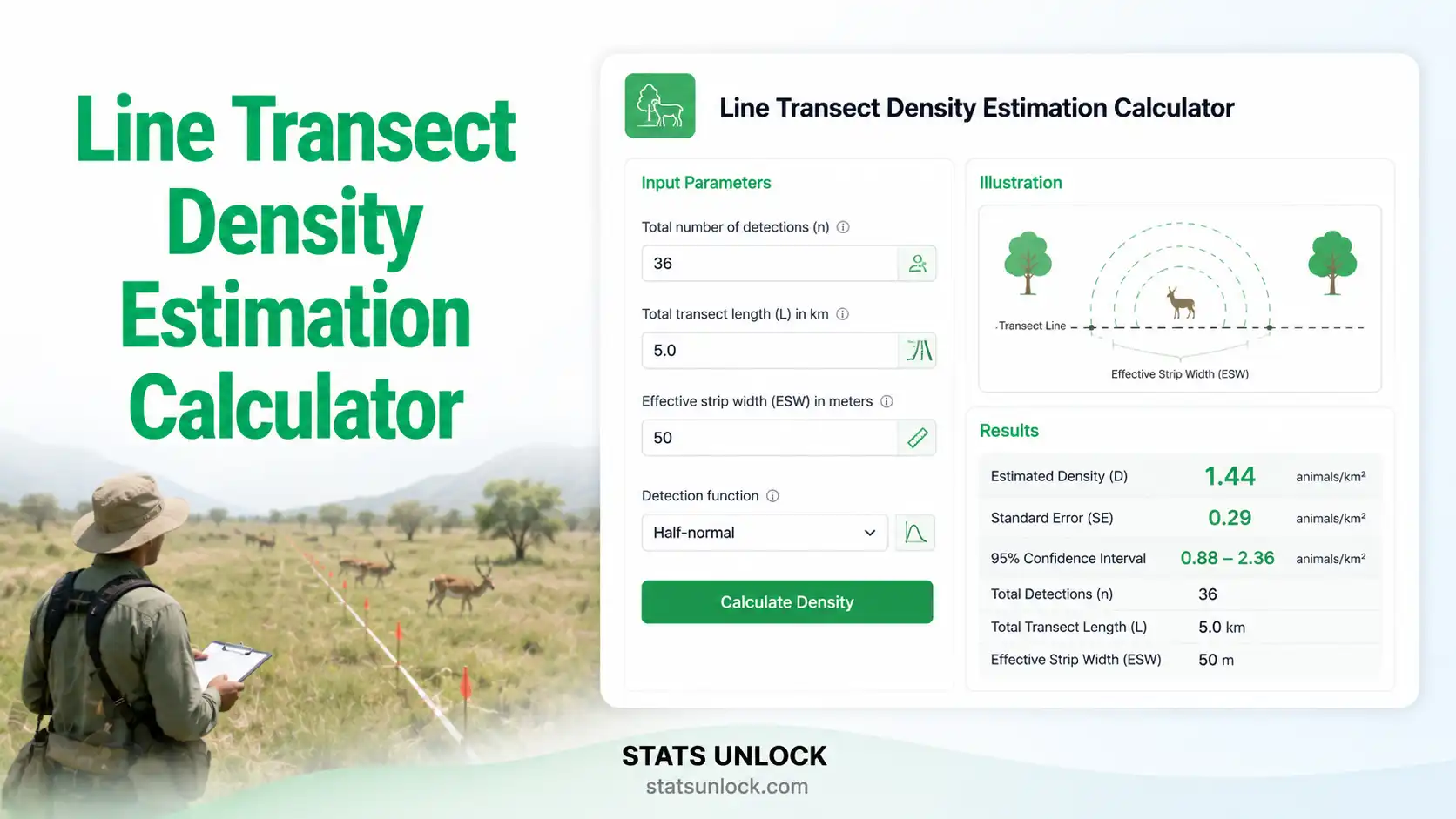
Line Transect Density Estimation Calculator
Free online wildlife population estimation tool using distance sampling. Calculate animal density, effective strip width, detection probability, encounter rate, and 95% confidence intervals for single or multiple species.
🚶 How Line Transect Data Is Collected
Observers walk along a straight transect line and record the perpendicular distance from the line to every detected animal within a truncation half-width w. Animals closer to the line are detected with higher probability than animals farther away — the detection function g(x) models this falloff. The tool fits g(x), computes the average detection probability Pa within the strip, and converts the count into a density estimate.
📖 How this diagram maps to the analysis
Step 1 — Field protocol. Observer walks a pre-set transect line of length L at a constant pace, recording every detection within the truncation half-width w on either side. Distance is measured perpendicular from the line to where the animal was first seen (not the slant distance from the observer).
Step 2 — Data structure. Each row in your CSV / textarea is one detection: a numeric perpendicular distance in meters. With total length L and n total detections, you have one column of distances per species (multi-species mode) or one combined column (single-species mode).
Step 3 — What the tool calculates. The tool fits a detection function g(x) to the histogram of perpendicular distances. The model parameters give the average detection probability Pa within the truncated strip. Density is then estimated as D̂ = n · E(s) / (2 · w · L · Pa).
Step 4 — Why truncation matters. Animals beyond w are excluded because detection at long distances is unreliable and can destabilise the model fit. Choose w so that approximately 5–10% of detections are truncated (Buckland et al. 2001).
📊 Data Input
Comma-separated input (default). Format: 52, 48, 55, 61, 47, ... — one detection distance per value, in meters.
Enter detection distances row-by-row. Click "Add Row" for more entries, then click "Use This Data" to load.
| # | Distance (m) |
|---|
Download Sample Data
Try the tool with real-world example datasets — includes multi-species CSV files, README, and instructions for USA wildlife (deer, bear, turkey, coyote, cottontail).
⚙️ Survey Configuration
Enter the value in your chosen units (right →). Default: 50 km.
Choose any unit — internally converted to meters.
Default: Half-Normal. Use "Auto-Select" to fit all key functions and pick the lowest-AIC model.
Choose the area unit appropriate to your study (USA defaults: per km² or per mi²).
📈 Analysis Results
Line Transect Density Equation
The animal density (D̂) is estimated from distance sampling theory:
- D̂: estimated animal density (animals per unit area, e.g., per km²)
- n: total number of detections (groups or clusters)
- E(s): expected cluster size (mean group size)
- w: truncation half-width of the strip (m)
- L: total transect length surveyed (m or km)
- Pa: probability of detection within the truncation strip
- ESW: effective strip half-width = w × Pa
- μ: detection function shape parameter (half-normal σ)
📋 Detailed Results
📊 Visualizations
💡 Click any chart to download it as a 16:9 publication-ready PNG — 2560 × 1440 px (QHD), white background, embedded title and caption. Perfect for journals, slide decks, and posters.
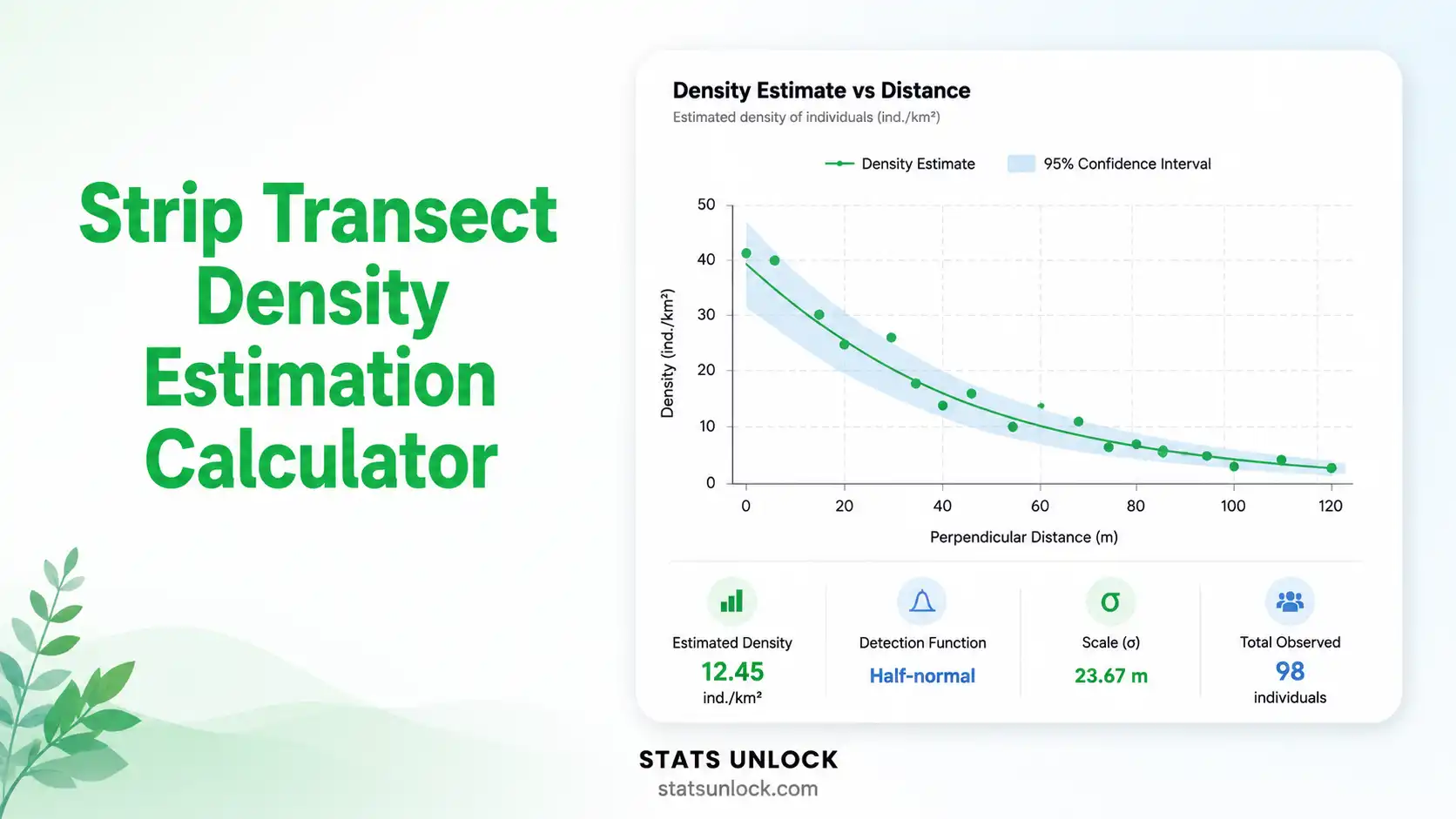
🎯 Detection Function Curve
Probability of detection vs perpendicular distance from transect line.
📏 Distance Distribution Histogram
Frequency of detections within distance bins.
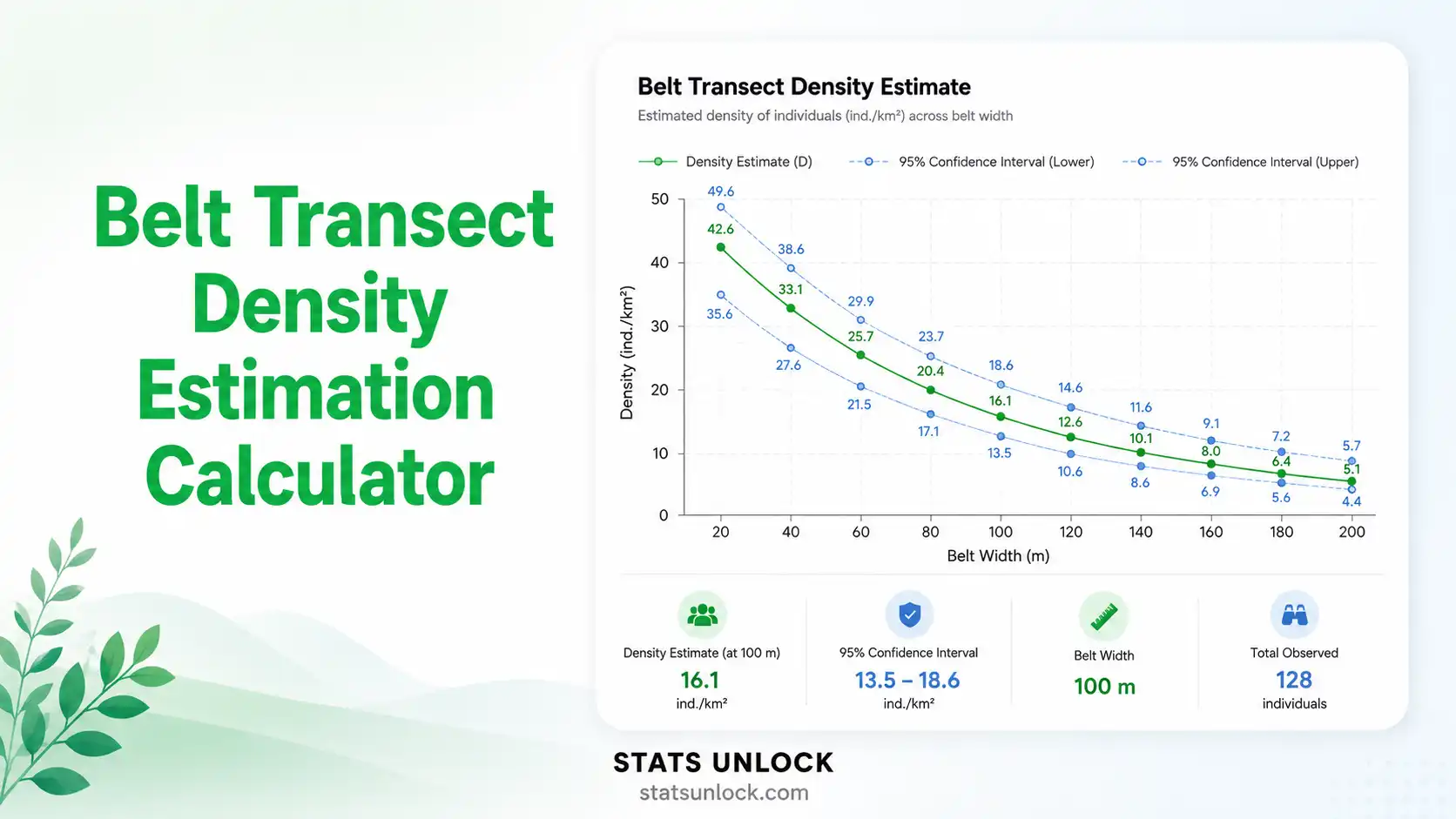
📊 Density Estimate with 95% CI
Bar = D̂ point estimate. Whiskers = 95% lower & upper CI. Multi-species runs add a dark "Community Total" bar. Hover for exact LCL/UCL.
🔍 Cumulative Detection Profile
Cumulative proportion of detections vs distance (used to verify shoulder).
📐 Methodology
Run the analysis above to generate the full methodology with citations, parameter values, and software-ready Methods text.
🧭 Detailed Interpretation of Results
Run the analysis above to generate the full detailed interpretation.
✍️ How to Write Your Results in Research
Run the analysis above to auto-fill five publication-ready reporting templates.
🪧 Research Poster Panel
Run the analysis above to generate a complete, attractively-designed research poster.
🎯 Detailed Conclusion
Run the analysis above to generate a full multi-section conclusion.
📐 Technical Notes & Formula Derivation
Show full formula derivation, assumptions, and limitations
Distance sampling foundation (Buckland et al. 2001): Line transect surveys assume animals are distributed independently of the transect line. Observers walk the line and record perpendicular distances (x) to every detected animal or group. Detection probability g(x) declines with distance, and the detection function is fit to the observed distance distribution.
Half-normal detection function: g(x) = exp(−x² / (2σ²)). The scale parameter σ is estimated by maximum likelihood from observed distances. ESW = σ × √(π/2).
Density formula derivation: Total animals within strip 2wL = N. Detected = n = N × Pa. Therefore N̂ = n / Pa and D̂ = N̂ / (2wL) = n / (2 × w × L × Pa) = n / (2 × ESW × L) for unit clusters.
Three core assumptions: (1) Animals on the transect line are detected with certainty — g(0) = 1. (2) Animals are detected at their original positions before any movement in response to the observer. (3) Perpendicular distances are measured accurately and without rounding bias.
Limitations: Violations of g(0) = 1 (missed animals on the line) systematically bias density downward. Heaping at zero or rounding distances flattens the detection function shoulder. Small sample sizes (n < 60) produce wide CIs. Habitat-specific stratification is recommended when detection varies by cover.
Variance estimation: The variance of D̂ is approximated by var(D̂) = D̂² × (CVn² + CVPa² + CVE(s)²). Log-normal 95% confidence intervals are reported.
🎯 Detection Functions Reference (8 Models)
This calculator supports eight detection functions covering all standard families from Buckland et al. (2001). Each is fit by maximum likelihood; "Auto-Select Best Model" fits all eight and chooses the lowest-AIC model. The detection function g(x) describes how the probability of detecting an animal declines with perpendicular distance x from the transect line.
1️⃣ Half-Normal (Key Function)
Use when: the histogram of distances shows a wide flat shoulder near the line then a smooth Gaussian-like decline. The default for most line transect studies — robust, well-behaved, single-parameter. ESW = σ × √(π/2).
Parameters: σ (scale). k = 1.
2️⃣ Hazard-Rate (Key Function)
Use when: detection stays near 1.0 across a strong shoulder, then drops abruptly. Two-parameter, flexible shape. Common for visual aerial surveys of ungulates and marine mammals where detection is binary up to a threshold.
Parameters: σ (scale), b (shape). k = 2.
3️⃣ Uniform (Key Function)
Use when: detection is essentially perfect within w (strip transect equivalent). Useful as a null baseline for AIC comparison or with adjustment terms. ESW = w, Pa = 1.
Parameters: none. k = 0.
4️⃣ Negative Exponential
Use when: detection declines exponentially from the line with no shoulder. Single-parameter. Often used for cue-counting surveys (calls, songs) where probability decays from the source. ESW = σ.
Parameters: σ (rate). k = 1.
5️⃣ Half-Normal + Cosine
Use when: the half-normal fit is close but the residuals show systematic deviation. Cosine series adds flexibility around the shoulder. Two parameters (σ, a₁).
Parameters: σ, a₁. k = 2.
6️⃣ Hazard-Rate + Simple Polynomial
Use when: hazard-rate fits the rough shape but a quadratic adjustment improves fit at intermediate distances. Three parameters give maximum flexibility — beware over-fitting with small n.
Parameters: σ, b, a₁. k = 3.
7️⃣ Uniform + Cosine
Use when: wide shoulder followed by gradual decline near w. Often the most parsimonious shape for small-mammal pitfall or transect surveys. One free parameter (a₁).
Parameters: a₁. k = 1.
8️⃣ Uniform + Hermite Polynomial
Use when: the data show subtle multi-modal departures from uniform that simple cosine cannot capture. The Hermite series is recommended by Buckland for more complex shoulder shapes.
Parameters: a₁. k = 1.
🏆 How to Choose: AIC Model Selection
Akaike Information Criterion (AIC = −2·logL + 2k) balances model fit against complexity. Lower is better. Rules of thumb (Burnham & Anderson 2002):
- Δ AIC < 2: models are essentially equivalent — prefer the simpler one
- Δ AIC = 2–4: alternative is plausible
- Δ AIC = 4–10: considerably less support
- Δ AIC > 10: essentially no support — drop from consideration
Select "Auto-Select Best Model (AIC)" in the Survey Configuration dropdown to fit all eight functions and automatically pick the lowest-AIC model. The full ranking table will appear under the results.
📋 Quick-Pick Guide by Survey Type
| Survey Type | Best Detection Function |
|---|---|
| Ungulate ground transect (deer, elk) | Half-Normal or Hazard-Rate |
| Aerial survey (helicopter / drone) | Hazard-Rate |
| Bird point-count / song surveys | Negative Exponential or Half-Normal |
| Small-mammal transect | Uniform + Cosine |
| Marine mammal boat survey | Hazard-Rate + Simple Polynomial |
| Strip transect baseline | Uniform |
| Unknown / pilot survey | Auto-Select Best Model (AIC) ✓ |
✅ When to Use Line Transect Density Estimation
Line transect is the gold standard for estimating wildlife density across large open or semi-open habitats in the USA and globally.
✓ Use when:
- ✓ Surveying ungulates (white-tailed deer, mule deer, pronghorn, elk) across rangelands or forests
- ✓ You can measure or estimate perpendicular distances reliably (≥ 60 detections per species)
- ✓ Habitat permits walking or driving a straight transect line
- ✓ Detection probability declines with distance but is high on the line
- ✓ You need absolute density (animals/km²) rather than relative indices
✗ Do NOT use when:
- ✗ Animals respond to observer presence before detection (use point transects or cameras)
- ✗ Sample size is very small (n < 30) — switch to mark-recapture or occupancy
- ✗ Habitat blocks straight-line walking (dense swamp, cliff terrain)
- ✗ Animals are highly clumped at scales smaller than the transect spacing
🌎 Real-world USA examples:
- White-tailed deer density in Pennsylvania state forests (Game Commission line transects)
- Pronghorn surveys in Wyoming sagebrush steppe (BLM aerial line transects)
- Mule deer monitoring in Colorado mountain parks (CPW spotlight transects)
- Wild turkey distance sampling in Texas Hill Country (TPWD ground transects)
📘 How to Use This Tool
- Choose your survey mode — Single Species (one animal) or Multi-Species (multiple animals on the same transect).
- Enter perpendicular detection distances — comma-separated meters, e.g.
52, 48, 55, 61, 47, ... - Optionally name your study area (e.g., "Yellowstone National Park") — auto-fills all reports and the research poster.
- Set total transect length (L) in km, mi, or m. USA users typically use km or mi.
- Set truncation distance (w) — drop distances beyond this (typical: 100–150 m for ungulates).
- Choose detection function — Half-Normal (default), Hazard-Rate, or Uniform+Cosine.
- Set output unit — per km², per mi² (USA), per ha, or per acre (USA).
- Click "Run Line Transect Analysis" to compute density, ESW, Pa, encounter rate, and 95% CI.
- Review the four visualizations — detection function, histogram, density CI, cumulative profile.
- Download Doc or PDF — full publication-ready report including poster, interpretation, and references.
❓ Frequently Asked Questions
What is line transect density estimation?
How do you calculate wildlife density from line transects?
What is effective strip width (ESW)?
What is the difference between line transect and strip transect?
How many detections are needed for line transect?
What detection functions are used in distance sampling?
What does Pa mean in line transect density?
What is the encounter rate in line transect surveys?
Can line transect be used for multiple species?
How accurate is line transect density estimation?
📚 References
Foundational and current peer-reviewed sources on line transect density estimation, distance sampling, and wildlife population estimation methods used in this calculator. Click any citation to open the source in a new tab.
- Buckland, S. T., Anderson, D. R., Burnham, K. P., Laake, J. L., Borchers, D. L., & Thomas, L. (2001). Introduction to Distance Sampling: Estimating Abundance of Biological Populations. Oxford University Press.
- Buckland, S. T., Rexstad, E. A., Marques, T. A., & Oedekoven, C. S. (2015). Distance Sampling: Methods and Applications. Springer.
- Thomas, L., Buckland, S. T., Rexstad, E. A., Laake, J. L., Strindberg, S., et al. (2010). Distance software: design and analysis of distance sampling surveys for estimating population size. Journal of Applied Ecology, 47(1), 5–14.
- Burnham, K. P., Anderson, D. R., & Laake, J. L. (1980). Estimation of density from line transect sampling of biological populations. Wildlife Monographs, 72, 3–202.
- Williams, B. K., Nichols, J. D., & Conroy, M. J. (2002). Analysis and Management of Animal Populations. Academic Press.
- Miller, D. L., Rexstad, E., Thomas, L., Marshall, L., & Laake, J. L. (2019). Distance Sampling in R. Journal of Statistical Software, 89(1), 1–28.
- Anderson, D. R., Laake, J. L., Crain, B. R., & Burnham, K. P. (1979). Guidelines for line transect sampling of biological populations. Journal of Wildlife Management, 43(1), 70–78.
- Marques, T. A., Thomas, L., Fancy, S. G., & Buckland, S. T. (2007). Improving estimates of bird density using multiple-covariate distance sampling. The Auk, 124(4), 1229–1243.
- U.S. Fish & Wildlife Service. (2022). Distance Sampling Protocol for Wildlife Surveys on National Wildlife Refuges. USFWS Technical Report.
- Pollock, K. H., Nichols, J. D., Simons, T. R., Farnsworth, G. L., Bailey, L. L., & Sauer, J. R. (2002). Large-scale wildlife monitoring studies: statistical methods for design and analysis. Environmetrics, 13(2), 105–119.
- Fewster, R. M., Buckland, S. T., Burnham, K. P., Borchers, D. L., Jupp, P. E., et al. (2009). Estimating the encounter rate variance in distance sampling. Biometrics, 65(1), 225–236.
- Marques, F. F. C., & Buckland, S. T. (2003). Incorporating covariates into standard line transect analyses. Biometrics, 59(4), 924–935.
- U.S. Geological Survey. (2020). Wildlife Population Estimation Field Manual. USGS Patuxent Wildlife Research Center.
- Texas Parks & Wildlife Department. (2023). Distance Sampling Guidelines for White-tailed Deer Population Surveys. TPWD Wildlife Division.
- Colorado Parks & Wildlife. (2022). Mule Deer Population Monitoring: Distance Sampling Protocol. CPW Wildlife Research.
- Akaike, H. (1973). Information theory and an extension of the maximum likelihood principle. In B. N. Petrov & F. Csáki (Eds.), Second International Symposium on Information Theory (pp. 267–281). Akadémiai Kiadó.
- Burnham, K. P., & Anderson, D. R. (2002). Model Selection and Multimodel Inference: A Practical Information-Theoretic Approach (2nd ed.). Springer.
- Buckland, S. T., Laake, J. L., & Borchers, D. L. (2010). Double-observer line transect methods: Levels of independence. Biometrics, 66(1), 169–177.
- Marsh, H., & Sinclair, D. F. (1989). Correcting for visibility bias in strip transect aerial surveys of aquatic fauna. Journal of Wildlife Management, 53(4), 1017–1024.
- Abramowitz, M., & Stegun, I. A. (1965). Handbook of Mathematical Functions with Formulas, Graphs, and Mathematical Tables. Dover Publications.
- Borchers, D. L., Buckland, S. T., & Zucchini, W. (2002). Estimating Animal Abundance: Closed Populations. Springer-Verlag.
- Marques, T. A., & Buckland, S. T. (2004). Covariate models for the detection function. Journal of Applied Ecology, 41(2), 366–377.
- Reynolds, R. T., Scott, J. M., & Nussbaum, R. A. (1980). A variable circular-plot method for estimating bird numbers. The Condor, 82(3), 309–313.
- Royle, J. A., Dawson, D. K., & Bates, S. (2004). Modeling abundance effects in distance sampling. Ecology, 85(6), 1591–1597.
- The Wildlife Society. (2020). Standards and Methods for Population Estimation in Wildlife Management. TWS Technical Review 20-01.