What does a high vs low density value mean?

High density (>1 individual per m² for herbs, >0.1 per m² for shrubs) indicates an abundant population, often a dominant or invasive species. Low density (<0.01 per m²) may indicate a rare species, edge of distribution, recent disturbance, or unsuitable habitat. Interpretation depends on growth form.

How do I report belt transect density in a research paper?

Report the mean density (per hectare and per m²), standard error, 95% confidence interval, sample size (number of replicate transects), and total area surveyed. Example: 'Mean density of Quercus alba was 412 ± 38 stems/ha (mean ± SE, n = 12 transects)'.

Can I use this tool for a thesis or peer-reviewed paper?

Yes, for exploratory and educational analysis. For final publication, verify results using R packages such as 'vegan' or 'unmarked' and cite both this calculator and the underlying methodology (Krebs 1999; Bonham 2013).

My density value seems unusually high — what could be wrong?

Common causes: double counting individuals, incorrect strip width (e.g., entering 1 m when it was 10 m), counting individuals outside the strip boundary, or including dead/last-year stems. Verify your raw counts and strip dimensions, then re-run.

Belt Transect Density Estimation Calculator — Free Online Vegetation Analysis Tool

📥 Data Input

Group Name (editable): Use Sample Dataset:

Counts per Transect Segment (comma-separated):

Enter each segment count separated by commas or new lines.

Upload CSV or Excel file:

Supports .csv, .txt, .xlsx, .xls — headers detected automatically.

Add segments manually as a small table:

Segment	Count

⚙️ Transect Configuration

Study Area / Site Name (optional):

Transect Width (m):

Typical: 1 m (herbs), 2 m (shrubs), 10 m (trees)

Segment Length (m):

Length of each individual segment

Area Output Unit:

Confidence Level:

📊 Density Estimation Summary

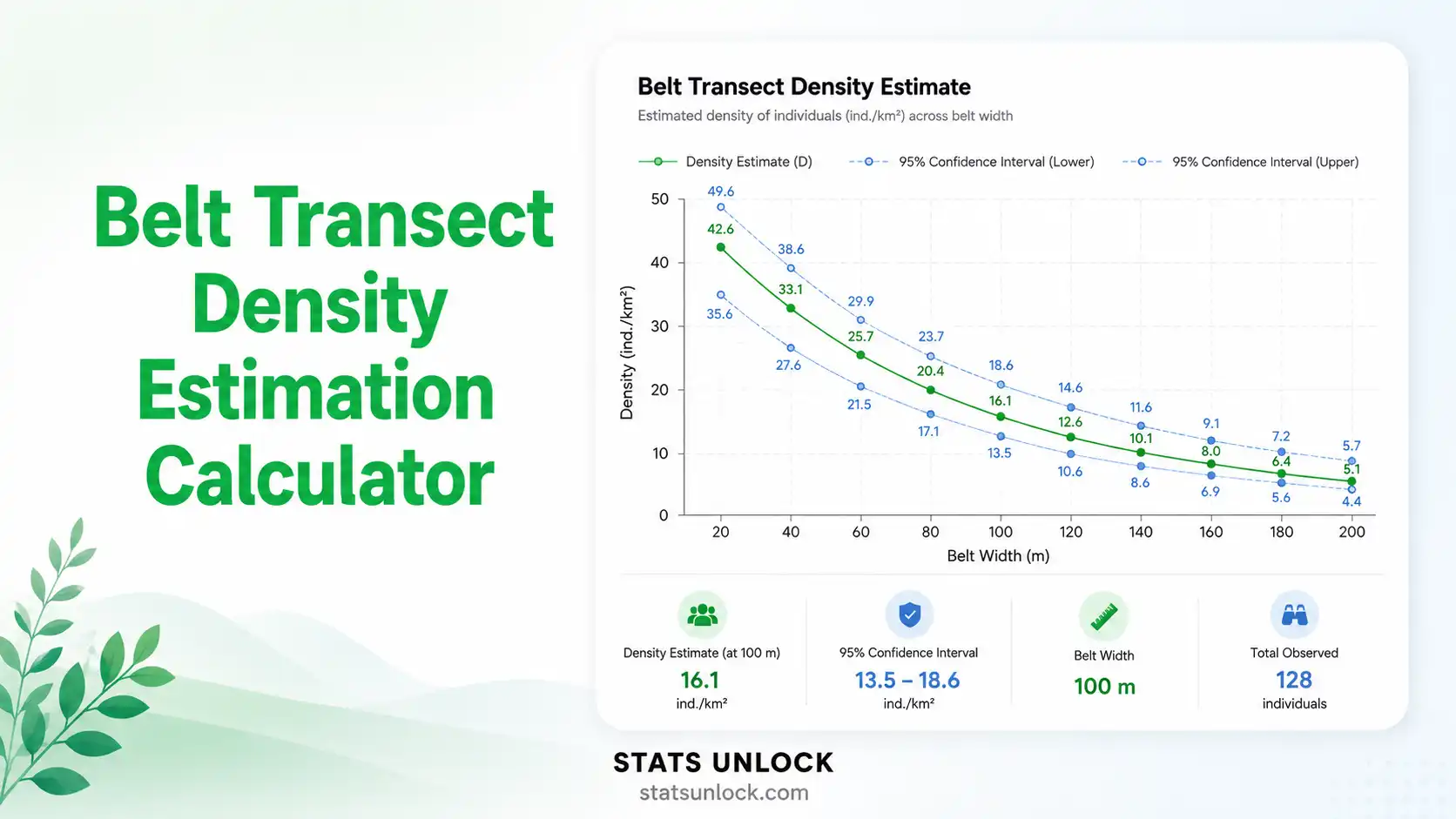
Belt Transect Density Equation

The fundamental formula for belt transect density (D) is:

D = NL × W

where the total surveyed area = L × W

D: Density (individuals per unit area, e.g., per m² or per hectare)
N: Total number of individuals counted across all transect segments
L: Total length of the transect line (m) — segment length × number of segments
W: Full width of the belt (m) — the value entered in the "Transect Width" field
SE: Standard error = s / √n, where s = sample standard deviation of segment-level densities, n = number of segments
95% CI: Mean ± (t_{α/2, n-1} × SE)

Statistic	Value	Description

📊 Count per Segment

📈 Cumulative Detection Curve

🎯 Density with 95% CI

📉 Frequency Distribution

📎 Copy Summary to Clipboard

🧭 Interpretation of Results

✍️ How to Write Your Results in Research

Five publication-ready templates plus a Research Poster Panel, all auto-filled with your current values. Click "📋 Copy" to use any template instantly.

🎯 Detailed Conclusion

📐 Technical Notes — Formula Derivation, Assumptions, Limitations

Extended Formula Derivation

Belt transect density is derived from the simple plot-based density estimator. A belt transect is essentially a long, narrow rectangular plot of area A = L × W, where W is the full transect width. The maximum-likelihood estimator of density is:

D̂ = N / A = N / (L × W)

For replicate transects or segments of equal length, the per-segment density d_i = n_i / (l_i × W). The mean density across k segments is:

D̄ = (1/k) Σ d_i

Standard error: SE(D̄) = s_d / √k, where s_d is the sample standard deviation of segment-level densities.

Assumptions

Perfect detection: All individuals within the strip are detected — detection probability = 1
Random or systematic placement: Transects are placed without bias toward areas of higher abundance
Closure: The population is closed (no births/deaths/migration) during sampling
Independence: Segments are independent samples (sufficient distance between them)
Constant width: The strip width is uniformly applied and accurately measured

Limitations

Detection bias: cryptic, small, or buried individuals are undercounted — leads to underestimation of true density
Edge effects: individuals straddling the boundary create ambiguity; standard rule is "include if center is inside"
Habitat heterogeneity: a single transect may not capture spatial variation — replicate transects are essential
Observer effects: training and experience strongly influence count accuracy in dense vegetation
Strip width sensitivity: incorrect width assumptions cause proportional bias in density estimates

📌 When to Use This Tool

Decision Checklist

✅ You have count data of individuals along a defined rectangular strip
✅ Your strip width and segment length are known and standardized
✅ You want a density estimate per unit area (per m² or per hectare)
✅ Your target species is sessile (plants) or slow-moving (sea urchins, snails)
❌ Do NOT use if your species moves faster than you walk → use distance sampling instead
❌ Do NOT use if your strip width is unknown or detection probability is < 1 → use distance sampling
❌ Do NOT use if you only have presence/absence data → use occupancy modeling

Real-World Examples

Forestry — Tree Density Survey: 10 m × 100 m belts in Great Smoky Mountains National Park, TN, to estimate Quercus alba density across slope gradients
Rangeland Ecology — Sagebrush Monitoring: 2 m × 50 m belts in Yellowstone NP to track Artemisia tridentata recovery post-fire
Grassland Restoration — Prairie Plants: 1 m × 30 m belts in Konza Prairie LTER (KS, USA) to compare native bunchgrass density between burned and unburned patches
Coastal Ecology — Salt Marsh Cordgrass: 1 m × 20 m belts in Chesapeake Bay to monitor Spartina alterniflora stem density along elevation gradients

Sampling Design Guidance

Minimum: 5 replicate transects per habitat type; ≥ 30 total individuals counted
Stratify by habitat or environmental gradient before placement
Walk a fixed pace (e.g., 30 m/min) to standardize effort
Use rope or measuring tape to maintain consistent strip width

Related Metrics — Decision Tree

Need density per unit area for sessile organisms? → Belt Transect Density
  → All individuals detected within strip? → Belt Transect (this tool)
  → Detection probability decreases with distance? → Line Transect / Distance Sampling
  → Animals are mobile? → Mark-Recapture (Lincoln-Petersen, POPAN)
Need just presence/absence? → Occupancy Modeling (MacKenzie 2002)
Need species composition rather than density? → IVI / Relative Density
Need to compare communities? → Shannon-Wiener, Simpson's Diversity

📖 How to Use This Tool — Step-by-Step Guide

Enter Your Data — Use the Paste/Type tab with comma-separated counts (e.g., "52, 48, 55, 61, 47"). Each number is the count for one segment of the transect. Example: a 100 m transect divided into 10 segments of 10 m each gives 10 counts.
Choose a Sample Dataset — Five US ecological datasets are pre-loaded — pick one to see how the tool works on real-world vegetation data from Yellowstone, Konza Prairie, Chesapeake Bay, etc.
Configure Analysis Settings — Set the Transect Width (m), Segment Length (m), output unit, and confidence level. Example: 2 m width × 10 m segment length = 20 m² per segment.
Run the Analysis — Click "Calculate Belt Transect Density." The tool computes: total individuals (N), total area surveyed, mean density per m², density per ha, SE, and CI.
Read the Summary Cards — Green = high/healthy density, amber = moderate, red = low density / conservation concern. Density tier depends on growth form (herb vs tree).
Read the Full Results Table — All sub-components: count totals, density per unit area, SE, CI, CV (coefficient of variation), Z-test vs threshold.
Examine the Four Visualizations — Count per segment (bar), cumulative detection curve (line), density with 95% CI (error bar), frequency distribution (histogram).
Read the Ecological Interpretation — Five auto-filled paragraphs that translate your numbers into plain English suitable for park management reports or thesis chapters.
Copy a Reporting Example — Six ready-to-use templates: Ecology Journal, Thesis, Policy Brief, Conference Abstract, Monitoring Report, Research Poster.
Export Your Results — Download Doc (.txt) for sharing or Download PDF for printing your full report.

❓ Frequently Asked Questions

Q1. What is belt transect density estimation and when should I use it?

Belt transect density estimation is a vegetation sampling method that counts individuals of a target species within a rectangular strip of known length and width, then divides the count by the surveyed area to estimate density per unit area (e.g., per m² or per hectare).

Use it for plant population surveys, grassland monitoring, forest understorey assessments, coral reef benthos counts, and any sessile or slow-moving organism where you can confidently detect every individual inside the strip. It is the standard method taught in AP Biology, ecology lab courses, and field methods textbooks (Krebs 1999; Bonham 2013).

Q2. What data do I need for a belt transect density calculation?

You need: (1) counts of individuals for each transect segment or replicate, (2) the transect width in meters, and (3) the length of each segment (or the total transect length). Counts can be entered as a comma-separated list, one per line, in a column entry grid, or uploaded from a CSV/Excel file. Optional: a label for each segment, useful for plotting and reporting.

Q3. What does a high vs low belt transect density value mean ecologically?

Interpretation depends entirely on the growth form. For herbaceous plants, > 50 individuals/m² is high; for shrubs, > 0.5/m² is high; for canopy trees, > 0.05/m² (500/ha) is high. A high value usually indicates favorable habitat, abundant resources, or dominance/invasion. A low value may indicate disturbance, edge of distribution, unsuitable conditions, or recent harvest/fire. Always compare your value to published benchmarks for the same species and habitat.

Q4. How does belt transect density differ from quadrat sampling?

Quadrats are independent square plots placed randomly or systematically; belt transects are continuous rectangular strips along a line. Belt transects are better for capturing spatial gradients (e.g., forest interior to edge, elevation transitions). Quadrats are more efficient for evenly distributed populations and easier to install. Both yield density per unit area; results are directly comparable if total area sampled is equal.

Q5. What are the assumptions and limitations of belt transect density?

Assumptions: (a) every individual inside the strip is detected, (b) transects are placed without bias, (c) the population is closed during sampling, (d) strip width is uniform and accurate.

Limitations: detection bias for cryptic individuals, edge effects on the strip boundary, habitat heterogeneity within a single transect, observer experience. If detection is imperfect, switch to line-transect distance sampling (Buckland et al. 2001).

Q6. How long and wide should my belt transect be?

Standard widths: 1 m for herbaceous/forb species, 2 m for sub-shrubs and small woody plants, 5–10 m for shrubs, 10–20 m for canopy trees. Length depends on habitat heterogeneity — typically 20–50 m for small plots, 100–500 m for landscape-scale surveys. Aim for at least 30 total individuals counted across all transects/segments to make the estimate reliable.

Q7. Can I compare belt transect density between sites or years?

Yes — provided the strip width, segment length, observer protocols, and season are standardized across all surveys. Use independent-samples t-tests or ANOVA on the segment-level densities. If the assumptions of normality are violated (often the case with count data), use Mann-Whitney U or Kruskal-Wallis instead. Always report the standard error and 95% confidence interval, not just the point estimate.

Q8. How do I report belt transect density in an ecology journal or research paper?

Report: (1) the mean density per hectare and per m², (2) standard error or 95% CI, (3) number of replicate transects (n), (4) total area surveyed (m²), (5) growth form / species, (6) habitat description. Example: "Mean density of Quercus alba was 412 ± 38 stems/ha (mean ± SE, n = 10 transects, total area = 0.2 ha)." See Section 7 above for six complete reporting templates.

Q9. Can I use this calculator for a thesis or peer-reviewed publication?

Yes for exploratory and educational analysis. For final publication, we recommend verifying results with peer-reviewed statistical software such as the R package vegan (Oksanen et al. 2022) or unmarked (Fiske & Chandler 2011). Cite this tool as: StatsUnlock. (2026). Belt Transect Density Estimation Calculator. Retrieved from https://statsunlock.com.

Q10. My belt transect density value seems unexpectedly high or low — what could be wrong?

Common causes: (1) double-counting individuals straddling segment boundaries, (2) entering the wrong strip width (e.g., 1 m when it was 10 m — this changes density by 10×), (3) including dead or last-year stems, (4) outliers from a single high-count segment, (5) unequal sampling effort. Verify your raw counts and re-check the strip width before drawing conclusions. Try the sample datasets to confirm the tool is producing the expected values.

📚 References

The following references support the statistical and ecological methods used in this belt transect density estimation calculator, covering vegetation sampling, plant density estimation, and best practices in field ecology methodology.

Krebs, C. J. (1999). Ecological methodology (2nd ed.). Benjamin Cummings. krebs.ubc.ca
Bonham, C. D. (2013). Measurements for terrestrial vegetation (2nd ed.). Wiley-Blackwell. https://doi.org/10.1002/9781118534540
Buckland, S. T., Anderson, D. R., Burnham, K. P., Laake, J. L., Borchers, D. L., & Thomas, L. (2001). Introduction to distance sampling: Estimating abundance of biological populations. Oxford University Press. global.oup.com
Elzinga, C. L., Salzer, D. W., & Willoughby, J. W. (1998). Measuring & monitoring plant populations. BLM Technical Reference 1730-1. blm.gov/Library_BLMTechnicalReference1730-1
Cain, S. A. (1938). The species-area curve. The American Midland Naturalist, 19(3), 573–581. https://doi.org/10.2307/2420468
Burnham, K. P., & Anderson, D. R. (1980). Estimation of density from line transect sampling of biological populations. Wildlife Monographs, 72. jstor.org/stable/3830641
MacKenzie, D. I., Nichols, J. D., Royle, J. A., Pollock, K. H., Bailey, L. L., & Hines, J. E. (2017). Occupancy estimation and modeling (2nd ed.). Academic Press. https://doi.org/10.1016/C2012-0-01164-7
Oksanen, J., Simpson, G. L., Blanchet, F. G., et al. (2022). vegan: Community ecology package (R package version 2.6-4). CRAN.R-project.org/package=vegan
Fiske, I., & Chandler, R. (2011). unmarked: An R package for fitting hierarchical models of wildlife occurrence and abundance. Journal of Statistical Software, 43(10), 1–23. https://doi.org/10.18637/jss.v043.i10
Greig-Smith, P. (1983). Quantitative plant ecology (3rd ed.). Blackwell Scientific Publications.
Mueller-Dombois, D., & Ellenberg, H. (1974). Aims and methods of vegetation ecology. John Wiley & Sons.
Smith, D. W., Stahler, D. R., et al. (2020). Yellowstone Wolf Project Annual Report 2019. National Park Service. nps.gov/yell/wolf-report
R Core Team. (2024). R: A language and environment for statistical computing. R Foundation for Statistical Computing. https://www.R-project.org/
USDA Forest Service. (2020). Forest Inventory and Analysis National Core Field Guide. fia.fs.usda.gov
National Park Service. (2023). Vegetation monitoring protocols. Inventory & Monitoring Division. nps.gov/im/monitoring-vegetation