

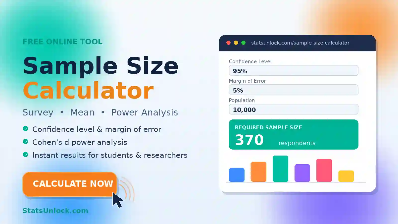

Sample Size Calculator: How Many Responses or Participants Do You Need?
Free sample size calculator for surveys, measurements, and two-group studies. Set your confidence level, margin of error, and population size, and get the minimum sample instantly — with the Cochran formula, finite population correction, Slovin's formula, power analysis, four charts, and copy-ready sentences for your methods section.
Quick answer: The survey sample size formula is n = z² p(1−p) ÷ e². At 95% confidence (z = 1.96), a 5% margin of error, and p = 0.5, you need 385 completed responses — for almost any population size. For a 3% margin you need about 1,068; for 2%, about 2,401. Small known populations need fewer (finite population correction).
🔑 Key Takeaways
- 1385 is the magic survey number. At 95% confidence with a 5% margin of error, 385 responses is enough whether your population is 10 thousand or 10 million.
- 2Population size barely matters once it is large. Required n levels off fast — the finite population correction only helps when you sample a noticeable fraction of a small population.
- 3Precision is expensive: n grows with 1/e². Halving the margin of error (5% → 2.5%) roughly quadruples the sample you need.
- 4Use p = 0.5 when the proportion is unknown. It maximizes p(1−p) and therefore gives the safest, most conservative sample size.
- 5Comparing groups? Use power analysis, not the survey formula. n per group = 2(zα/2 + zpower)² / d² — about 63 per group for a medium effect (d = 0.5) at 80% power.
- 6Plan for non-response. The formulas give completed responses; divide by your expected response rate (e.g., 385 ÷ 0.40 ≈ 963 invitations at a 40% response rate).
- 7Slovin's formula is a quick shortcut, not a replacement. n = N/(1+Ne²) silently assumes 95% confidence and p = 0.5 — fine for coursework, but report Cochran's formula in serious research.
🧮 Calculate Your Sample Size
🛠 How to Use This Sample Size Calculator
- Pick the goal. Survey / Proportion for polls and questionnaires, Estimating a Mean for measurements, or Comparing Two Groups for experiments and clinical trials — or load one of the ten sample scenarios.
- Set the confidence level. 95% is standard; choosing 99% grows the sample, 90% shrinks it.
- Set the margin of error. 5% is typical for surveys. Remember the inverse-square rule: halving the margin quadruples the sample.
- Add the population size if it is small and known. The finite population correction can substantially cut the required sample for populations under a few thousand.
- Click "Calculate Sample Size." You get the minimum n, the Slovin comparison, invitations needed after non-response, and four charts of the trade-offs — then copy a methods-section sentence from the reporting templates below.
📑 Sample Size Table: Common Survey Scenarios at a Glance
These are the numbers everyone looks up, computed with the Cochran formula (p = 0.5) and the finite population correction. Rows are population sizes; columns are margins of error at 95% confidence.
| Population (N) | ±10% margin | ±5% margin | ±3% margin | ±2% margin |
|---|---|---|---|---|
| 100 | 50 | 80 | 92 | 97 |
| 500 | 81 | 218 | 341 | 414 |
| 1,000 | 88 | 278 | 517 | 707 |
| 5,000 | 94 | 357 | 880 | 1,623 |
| 10,000 | 95 | 370 | 965 | 1,937 |
| 100,000 | 96 | 383 | 1,056 | 2,345 |
| 1,000,000+ | 97 | 385 | 1,067 | 2,401 |
Notice how each column flattens as N grows — that is why "how big is the population?" matters far less than "how precise do you need to be?". The z-values behind this table are 1.645 (90%), 1.960 (95%), and 2.576 (99%).
ƒ Sample Size Formulas Used
🔍 Interpreting Your Sample Size — In Detail
The number this calculator returns is the minimum number of completed, usable responses or measurements needed to hit your stated precision or power. Three trade-offs govern it, and understanding them lets you negotiate with reviewers, clients, and budgets.
The three levers
Margin of error is the dominant lever. Because n scales with 1/e², tightening the margin from ±5% to ±3% takes you from 385 to 1,068 responses, and ±2% demands 2,401. If a survey budget is fixed, relax the margin rather than the confidence level. Confidence level is the second lever: moving from 95% to 99% multiplies the sample by (2.576/1.960)² ≈ 1.73. Population size is the weakest lever: it only helps when the population is small — at N = 500 a 5%-margin survey needs just 218 respondents instead of 385, but past N ≈ 20,000 the correction is negligible.
Reading the power analysis result
For two-group comparisons, the output is per group, so double it for the total. The driving force is the effect size you want to detect: small effects are brutally expensive (d = 0.2 needs ~394 per group at 80% power) while large effects are cheap (d = 0.8 needs ~26). If your computed sample is unaffordable, your realistic options are accepting detection of only larger effects, raising α (rarely acceptable), lowering power (risky — 80% is already the conventional floor), or using a stronger design (paired measurements, ANCOVA with covariates, or more precise instruments).
What the number does not fix
Sample size buys precision, not validity. A perfectly sized sample drawn from a biased frame (only daytime landline answerers, only volunteers) still misestimates the population — non-random selection error does not shrink with n. Likewise the formulas assume simple random sampling; cluster and stratified designs need a design-effect multiplier (commonly 1.5–2.0 for cluster samples). And remember the result counts completes: always inflate by your expected response rate before sending invitations.
✍ How to Write Sample Size in Your Methods Section
Journals and thesis committees expect an explicit sample size justification. Below are copy-ready templates — replace the bracketed values with your numbers from the results table above.
Template 1 — Survey (Cochran + FPC)
Template 2 — Slovin's formula
Template 3 — Estimating a mean
Template 4 — Power analysis (two groups)
Reporting checklist
State the formula or software used; report every input (confidence level or α, margin of error or effect size, power, assumed proportion or SD, population size); justify the effect size or SD with a citation or pilot data; describe the rounding and any inflation for non-response or attrition; and name the sampling method, since the formulas assume simple random sampling.
🔬 Example Results
Six worked examples matching the sample scenarios in the dropdown above. Load any scenario and click Calculate to reproduce the numbers exactly.
Example 1 — Standard Survey: The Famous 385
n₀ = 1.96² × 0.25 ÷ 0.05² = 384.16 → n = 385
The most-quoted number in survey research. With no population entered, the Cochran formula alone applies. The curve shows why pollsters settle at ±5%: pushing to ±2% costs six times the respondents.
Example 2 — Customer Survey with a Known Population (N = 5,000)
FPC: 384.16 ÷ [1 + 383.16/5000] = 356.9 → n = 357
The finite population correction trims 385 down to 357 — a modest saving at N = 5,000. At a 40% response rate you would send 357 ÷ 0.40 ≈ 893 invitations.
Example 3 — Small Employee Population (N = 350)
FPC: 384.16 ÷ [1 + 383.16/350] = 183.4 → n = 184
With only 350 employees, the correction is dramatic: 184 responses suffice instead of 385. This is where entering the population size genuinely pays off — you are surveying more than half the company either way.
Example 4 — Slovin's Formula for a Village Survey (N = 800)
Slovin: 800 ÷ (1 + 800 × 0.0025) = 266.7 → n = 267
Cochran + FPC: n = 260
Slovin's shortcut and the full Cochran calculation land within a few respondents of each other — because Slovin secretly assumes exactly the Cochran defaults (95%, p = 0.5). Use whichever your committee expects, and cite it.
Example 5 — Estimating Mean IQ (σ = 15, e = ±3)
n = (1.96 × 15 ÷ 3)² = 96.04 → n = 97
To pin the population mean IQ within ±3 points at 95% confidence, 97 participants suffice. Tighten to ±2 points and the requirement jumps to 217 — the inverse-square rule again, this time on the measurement scale.
Example 6 — Power Analysis: Two-Group Trial (d = 0.5, 80% Power)
n = 2 × (1.960 + 0.8416)² ÷ 0.5² = 62.8 → 63 per group (126 total)
The classic clinical-trial calculation. Detecting a medium effect needs 63 participants per arm; halving the effect size to d = 0.25 would need roughly four times as many. Add ~10% for expected dropout when recruiting.
🧭 When to Use This Tool
Use this sample size calculator whenever you are planning a survey or questionnaire and need to know how many responses make it representative, designing an experiment or clinical trial and must justify participants per group, estimating a population mean to a stated precision, writing the sample-size paragraph of a thesis or grant proposal, checking a published study's power after the fact, or teaching sample size determination, Slovin's formula, or power analysis. It fits researchers, students, market researchers, UX teams sizing A/B tests, and anyone who must defend the question "why n = 385?"
⚠ Assumptions & Limitations
All formulas here assume simple random sampling; stratified designs need slightly fewer and cluster designs need more (multiply by a design effect, typically 1.5–2.0 for cluster surveys). The proportion formula uses the normal approximation, which weakens when n×p or n×(1−p) is below about 10 — for very rare outcomes use exact binomial methods. The mean formula requires an estimate of σ; if it comes from a small pilot, treat the result as a floor and add a safety margin. Power calculations depend entirely on the effect size you assume — an optimistic d produces an underpowered study, which is the single most common design failure in published research (Button et al., 2013). The outputs count completed, usable observations: inflate for non-response, attrition, and invalid records. Finally, no sample size can repair a biased sampling frame — representativeness comes from how you sample, not how many you sample.
🏁 Conclusion
Sample size determination comes down to one honest question: how wrong can you afford to be? Translate that tolerance into a margin of error (or a minimum detectable effect), fix your confidence level or power, and the formulas do the rest. For surveys, the Cochran formula with p = 0.5 gives the safe answer — 385 completes for ±5% at 95% confidence — and the finite population correction earns real savings only for small populations. For measurements, sample size scales with (zσ/e)². For group comparisons, power analysis rules, and the effect size you choose is the assumption that deserves the most scrutiny.
Keep the three levers straight: margin of error is quadratic and dominates the cost; confidence level is a multiplier you rarely change; population size hardly matters once it is large. Then remember what the number cannot do — it cannot fix a biased frame, a leading questionnaire, or a lazy sampling method. A smaller random sample beats a larger convenience sample every time.
This calculator gives you the complete workflow: survey, mean, and power modes, Slovin's formula for comparison, non-response inflation, a lookup table of the classic scenarios, four trade-off charts, and methods-section sentences ready to paste. Decide your precision, press Calculate, and recruit with confidence — that is all sample size planning ever asks of you.
❓ Frequently Asked Questions
How do I calculate sample size for a survey?
What is a good sample size for a survey?
Why is 385 the standard survey sample size?
Does population size affect sample size?
What is Slovin's formula and when should I use it?
How does margin of error affect sample size?
What z-scores do the confidence levels use?
Why use 50% as the expected proportion?
What sample size do I need to compare two groups?
What is statistical power and why 80%?
What is Cohen's d and how do I choose it?
How do I account for non-response?
Is a larger sample always better?
What sample size is needed for qualitative research?
Do these formulas work for stratified or cluster sampling?
What is the finite population correction?
Why do I round the sample size up instead of normally?
How many responses do I need per survey question or subgroup?
What sample size do I need for an A/B test?
Can I calculate sample size after collecting the data?
📚 References
- Cochran, W. G. (1977). Sampling Techniques (3rd ed.). John Wiley & Sons. Publisher page
- Cohen, J. (1988). Statistical Power Analysis for the Behavioral Sciences (2nd ed.). Lawrence Erlbaum. https://doi.org/10.4324/9780203771587
- Cohen, J. (1992). A power primer. Psychological Bulletin, 112(1), 155–159. https://doi.org/10.1037/0033-2909.112.1.155
- Yamane, T. (1967). Statistics: An Introductory Analysis (2nd ed.). Harper & Row. Internet Archive
- Krejcie, R. V., & Morgan, D. W. (1970). Determining sample size for research activities. Educational and Psychological Measurement, 30(3), 607–610. https://doi.org/10.1177/001316447003000308
- Bartlett, J. E., Kotrlik, J. W., & Higgins, C. C. (2001). Organizational research: Determining appropriate sample size in survey research. Information Technology, Learning, and Performance Journal, 19(1), 43–50. Full text PDF
- Button, K. S., Ioannidis, J. P. A., Mokrysz, C., Nosek, B. A., Flint, J., Robinson, E. S. J., & Munafò, M. R. (2013). Power failure: Why small sample size undermines the reliability of neuroscience. Nature Reviews Neuroscience, 14(5), 365–376. https://doi.org/10.1038/nrn3475
- Faul, F., Erdfelder, E., Lang, A.-G., & Buchner, A. (2007). G*Power 3: A flexible statistical power analysis program. Behavior Research Methods, 39(2), 175–191. https://doi.org/10.3758/BF03193146
- Lakens, D. (2022). Sample size justification. Collabra: Psychology, 8(1), 33267. https://doi.org/10.1525/collabra.33267
- Kish, L. (1965). Survey Sampling. John Wiley & Sons. Publisher page
- Israel, G. D. (1992). Determining Sample Size (PEOD-6). University of Florida IFAS Extension. Full text PDF
- Charan, J., & Biswas, T. (2013). How to calculate sample size for different study designs in medical research? Indian Journal of Psychological Medicine, 35(2), 121–126. https://doi.org/10.4103/0253-7176.116232
- Noordzij, M., Tripepi, G., Dekker, F. W., Zoccali, C., Tanck, M. W., & Jager, K. J. (2010). Sample size calculations: Basic principles and common pitfalls. Nephrology Dialysis Transplantation, 25(5), 1388–1393. https://doi.org/10.1093/ndt/gfp732
- Guest, G., Bunce, A., & Johnson, L. (2006). How many interviews are enough? An experiment with data saturation and variability. Field Methods, 18(1), 59–82. https://doi.org/10.1177/1525822X05279903
- Schoenfeld, D. A. (1983). Sample-size formula for the proportional-hazards regression model. Biometrics, 39(2), 499–503. https://doi.org/10.2307/2531021
- Lachin, J. M. (1981). Introduction to sample size determination and power analysis for clinical trials. Controlled Clinical Trials, 2(2), 93–113. https://doi.org/10.1016/0197-2456(81)90001-5
- Maxwell, S. E., Kelley, K., & Rausch, J. R. (2008). Sample size planning for statistical power and accuracy in parameter estimation. Annual Review of Psychology, 59, 537–563. https://doi.org/10.1146/annurev.psych.59.103006.093735
- NIST/SEMATECH. (2012). Sample sizes required. In e-Handbook of Statistical Methods. https://www.itl.nist.gov/div898/handbook/prc/section2/prc222.htm
- Daniel, W. W., & Cross, C. L. (2018). Biostatistics: A Foundation for Analysis in the Health Sciences (11th ed.). Wiley. Publisher page
- Moore, D. S., McCabe, G. P., & Craig, B. A. (2021). Introduction to the Practice of Statistics (10th ed.). W. H. Freeman. Publisher page